easyclimate.physics
Submodules
Functions
|
Calculate the Coriolis parameter at each point. |
|
Calculate the latitudes and weights used by the Lin-Rood model. |
|
Calculate the ambient dew point temperature given the vapor pressure. |
|
Calculate moist adiabatic lapse rate. |
|
Calculate the mixing ratio of a gas. |
|
Calculate the saturation mixing ratio of water vapor. |
|
Calculate the vapor pressure. |
|
Calculate the saturation water vapor (partial) pressure. |
|
Calculate wet-bulb potential temperature using iteration. |
Calculate wet-bulb potential temperature (\(\theta_w\)). |
|
Calculate wet-bulb potential temperature using Robert Davies-Jones (2008) approximation. |
|
|
Calculate wet-bulb temperature using Stull (2011) empirical formula. |
|
Calculate wet-bulb temperature using Sadeghi et. al (2011) empirical formula. |
|
Calculate equivalent potential temperature using Bolton (1980) approximation. |
Calculate equivalent potential temperature using Robert Davies-Jones (2009) approximation. |
|
|
Calculate the potential temperature for dry air. |
|
Calculate the potential temperature for vertical variables. |
|
Calculate virtual temperature. |
|
Calculate virtual temperature. |
Calculate lifting condensation level using Bolton (1980) approximation. |
|
Calculate lifting condensation level using Bohren & Albrecht (2023) approximation. |
|
|
Calculation of the Brunt-väisälä frequency for the vertical atmosphere. |
|
Calculate the static stability within a vertical profile. |
|
Calculate atmospheric enthalpy from temperature and humidity mixing ratio. |
|
Estimate latent heat flux for water: evaporization (condensation), melting (freezing) or sublimation (deposition). |
|
Calculate atmospheric relative angular momentum. |
Calculate the specific humidity from mixing ratio. |
|
Calculate the mixing ratio from specific humidity. |
|
|
Calculate the specific humidity from the dew point temperature and pressure. |
|
Calculate the mixing ratio from the dew point temperature and pressure. |
|
Calculate the dew point temperature from specific humidity and pressure. |
|
Calculate the relative humidity from dew point temperature. |
Calculate the relative humidity from mixing ratio, temperature, and pressure. |
|
Calculate the relative humidity from specific humidity, temperature, and pressure. |
|
|
Calculate dew point temperature from temperature and relative humidity. |
Package Contents
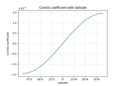
- easyclimate.physics.get_coriolis_parameter(lat_data: xarray.DataArray | numpy.array, omega: float = 7.292e-05) xarray.DataArray | numpy.array
Calculate the Coriolis parameter at each point.
\[f = 2 \Omega \sin(\phi)\]Parameters
- lat_data:
xarray.DataArrayornumpy.array. Latitude at each point.
- omega:
float, default: 7.292e-5 ( \(\mathrm{rad/s}\) ). The angular speed of the earth.
Returns
- Corresponding Coriolis force at each point ( \(\mathrm{s^{-1}}\) ).
xarray.DataArrayornumpy.array.
Reference
- lat_data:
- easyclimate.physics.calc_lat_weight_lin_rood(nlat: int) Tuple[numpy.ndarray, numpy.ndarray]
Calculate the latitudes and weights used by the Lin-Rood model.
The Lin-Rood model requires a specific distribution of latitudes and corresponding weights for numerical integration on a spherical grid. This function generates these values based on the number of desired latitudes.
Parameters
- nlat
int Number of latitudes. Must be at least 2 to define a valid grid (from pole to pole).
Returns
- Tuple[ndarray, ndarray]
A tuple containing two numpy arrays: - lat : ndarray
Array of latitudes in degrees, ranging from -90 (South Pole) to 90 (North Pole).
- weightndarray
Array of weights corresponding to each latitude, used for numerical integration.
Tip
The weights are computed such that they are suitable for use in the Lin-Rood semi-Lagrangian transport scheme. The latitudes are uniformly spaced between the poles.
References
Lin, S., & Rood, R. B. (1996). Multidimensional Flux-Form Semi-Lagrangian Transport Schemes. Monthly Weather Review, 124(9), 2046-2070. https://journals.ametsoc.org/view/journals/mwre/124/9/1520-0493_1996_124_2046_mffslt_2_0_co_2.xml
Lin, S.-J. and Rood, R.B. (1997), An explicit flux-form semi-lagrangian shallow-water model on the sphere. Q.J.R. Meteorol. Soc., 123: 2477-2498. https://doi.org/10.1002/qj.49712354416
- nlat
- easyclimate.physics.calc_dewpoint(vapor_pressure_data: xarray.DataArray, vapor_pressure_data_units: Literal['hPa', 'Pa', 'mbar']) xarray.DataArray
Calculate the ambient dew point temperature given the vapor pressure.
This function inverts the Bolton (1980) formula for saturation vapor pressure to instead calculate the temperature. This yields the following formula for dewpoint in degrees Celsius, where \(e\) is the ambient vapor pressure in millibars:
\[T = \frac{243.5 \log(e / 6.112)}{17.67 - \log(e / 6.112)}\]Parameters
- vapor_pressure_data:
xarray.DataArray. Water vapor partial pressure.
- vapor_pressure_data_units:
str. The unit corresponding to vapor_pressure_data value. Optional values are hPa, Pa.
Returns
- The dew point ( \(\\mathrm{degC}\) ).
See also
https://unidata.github.io/MetPy/latest/api/generated/metpy.calc.dewpoint.html
Bolton, D. (1980). The Computation of Equivalent Potential Temperature. Monthly Weather Review, 108(7), 1046-1053. https://journals.ametsoc.org/view/journals/mwre/108/7/1520-0493_1980_108_1046_tcoept_2_0_co_2.xml
- vapor_pressure_data:
- easyclimate.physics.calc_moist_adiabatic_lapse_rate(pressure_data: xarray.DataArray, temperature_data: xarray.DataArray, pressure_data_units: Literal['hPa', 'Pa', 'mbar'], temperature_data_units: Literal['celsius', 'kelvin', 'fahrenheit']) xarray.DataArray
Calculate moist adiabatic lapse rate.
Parameters
- pressure_data:
xarray.DataArray. The pressure data set.
- temperature_data:
xarray.DataArray. Atmospheric temperature.
- pressure_data_units:
str. The unit corresponding to pressure_data value. Optional values are hPa, Pa, mbar.
- temperature_data_units:
str. The unit corresponding to temperature_data value. Optional values are celsius, kelvin, fahrenheit.
Returns:
- dtdp
xarray.DataArray( \(\mathrm{K/hPa}\) ). Moist adiabatic lapse rate.
- pressure_data:
- easyclimate.physics.calc_mixing_ratio(partial_pressure_data: xarray.DataArray, total_pressure_data: xarray.DataArray, molecular_weight_ratio: float = 0.6219569100577033) xarray.DataArray
Calculate the mixing ratio of a gas.
This calculates mixing ratio given its partial pressure and the total pressure of the air. There are no required units for the input arrays, other than that they have the same units.
Parameters
- partial_pressure_data:
xarray.DataArray. Partial pressure of the constituent gas.
- total_pressure_data:
xarray.DataArray. Total air pressure.
- molecular_weight_ratio
float, optional. The ratio of the molecular weight of the constituent gas to that assumed for air. Defaults to the ratio for water vapor to dry air (\(\epsilon\approx0.622\)).
Note
The units of partial_pressure_data and total_pressure_data should be the same.
Returns
- The mixing ratio ( \(\mathrm{g/g}\) ).
- partial_pressure_data:
- easyclimate.physics.calc_saturation_mixing_ratio(total_pressure_data: xarray.DataArray, temperature_data: xarray.DataArray, temperature_data_units: Literal['celsius', 'kelvin', 'fahrenheit'], total_pressure_data_units: Literal['hPa', 'Pa', 'mbar']) xarray.DataArray
Calculate the saturation mixing ratio of water vapor.
This calculation is given total atmospheric pressure and air temperature.
Parameters
- total_pressure_data:
xarray.DataArray. Total atmospheric pressure.
- temperature_data:
xarray.DataArray. Atmospheric temperature.
- temperature_data_units:
str. The unit corresponding to temperature_data value. Optional values are celsius, kelvin, fahrenheit.
- total_pressure_data_units:
str. The unit corresponding to total_pressure_data value. Optional values are hPa, Pa.
Returns
- The saturation mixing ratio ( \(\mathrm{g/g}\) ).
- total_pressure_data:
- easyclimate.physics.calc_vapor_pressure(pressure_data: xarray.DataArray, mixing_ratio_data: xarray.DataArray, pressure_data_units: Literal['hPa', 'Pa', 'mbar'] = None, epsilon: float = 0.6219569100577033) xarray.DataArray
Calculate the vapor pressure.
Parameters
- pressure_data:
xarray.DataArray. The pressure data set.
- mixing_ratio_data:
xarray.DataArray. The mixing ratio of a gas.
- epsilon:
float. The molecular weight ratio, which is molecular weight of the constituent gas to that assumed for air. Defaults to the ratio for water vapor to dry air. (\(\epsilon \approx 0.622\))
- pressure_data_units:
str. The unit corresponding to pressure_data value. Optional values are hPa, Pa.
Returns
- The water vapor (partial) pressure, units according to
pressure_data_units.
- pressure_data:
- easyclimate.physics.calc_saturation_vapor_pressure(temperature_data: xarray.DataArray, temperature_data_units: Literal['celsius', 'kelvin', 'fahrenheit']) xarray.DataArray
Calculate the saturation water vapor (partial) pressure.
Parameters
- temperature_data:
xarray.DataArray. Atmospheric temperature.
- temperature_data_units:
str. The unit corresponding to temperature_data value. Optional values are celsius, kelvin, fahrenheit.
Returns
- The saturation water vapor (partial) pressure ( \(\mathrm{hPa}\) ).
See also
Bolton, D. (1980). The Computation of Equivalent Potential Temperature. Monthly Weather Review, 108(7), 1046-1053. https://journals.ametsoc.org/view/journals/mwre/108/7/1520-0493_1980_108_1046_tcoept_2_0_co_2.xml
https://unidata.github.io/MetPy/latest/api/generated/metpy.calc.saturation_vapor_pressure.html
- temperature_data:
- easyclimate.physics.calc_wet_bulb_temperature_iteration(temperature_data: xarray.DataArray, relative_humidity_data: xarray.DataArray, pressure_data: xarray.DataArray, temperature_data_units: Literal['celsius', 'kelvin', 'fahrenheit'], relative_humidity_data_units: Literal['%', 'dimensionless'], pressure_data_units: Literal['hPa', 'Pa', 'mbar'], A: float = 0.662 * 10**-3, tolerance: float = 0.01, max_iter: int = 100, method: Literal['easyclimate-backend', 'easyclimate-rust'] = 'easyclimate-rust') xarray.DataArray
Calculate wet-bulb potential temperature using iteration.
The iterative formula
\[e = e_{tw} - AP(t-t_{w})\]\(e\) is the water vapor pressure
\(e_{tw}\) is the saturation water vapor pressure over a pure flat ice surface at wet-bulb temperature \(t_w\) (when the wet-bulb thermometer is frozen, this becomes the saturation vapor pressure over a pure flat ice surface)
\(A\) is the psychrometer constant
\(P\) is the sea-level pressure
\(t\) is the dry-bulb temperature
\(t_w\) is the wet-bulb temperature
Parameters
- temperature_data:
xarray.DataArray. Atmospheric temperature.
- relative_humidity_data:
xarray.DataArray. The relative humidity.
- pressure_data:
xarray.DataArray. The pressure data set.
- temperature_data_units:
str. The unit corresponding to temperature_data value. Optional values are celsius, kelvin, fahrenheit.
- relative_humidity_data_units:
str. The unit corresponding to vapor_pressure_data value. Optional values are
%,dimensionless.- pressure_data_units:
str. The unit corresponding to pressure_data value. Optional values are hPa, Pa, mbar.
- A:
float. Psychrometer coefficients.
Psychrometer Type and Ventilation Rate
Wet Bulb Unfrozen (10^-3/°C^-1)
Wet Bulb Frozen (10^-3/°C^-1)
Ventilated Psychrometer (2.5 m/s)
0.662
0.584
Spherical Psychrometer (0.4 m/s)
0.857
0.756
Cylindrical Psychrometer (0.4 m/s)
0.815
0.719
Chinese Spherical Psychrometer (0.8 m/s)
0.7949
0.7949
- tolerance:
float. Minimum acceptable deviation of the iterated value from the true value.
- max_iter:
int. Maximum number of iterations.
- method{“easyclimate-backend”,”easyclimate-rust”}
Backend implementation.
Returns
- tw:
xarray.DataArray( \(\mathrm{degC}\) ) Wet-bulb temperature
Examples
>>> import xarray as xr
>>> import numpy as np

# Create sample data
>>> temp = xr.DataArray(np.array([20, 25, 30]), dims=['point'])
>>> rh = xr.DataArray(np.array([50, 60, 70]), dims=['point'])
>>> pressure = xr.DataArray(np.array([1000, 950, 900]), dims=['point'])

# Calculate wet-bulb potential temperature
>>> theta_w = calc_wet_bulb_potential_temperature_iteration(
...     temperature_data=temp,
...     relative_humidity_data=rh,
...     pressure_data=pressure,
...     temperature_data_units="celsius",
...     relative_humidity_data_units="%",
...     pressure_data_units="hPa"
... )

# Example with 2D data
>>> temp_2d = xr.DataArray(np.random.rand(10, 10) * 30, dims=['lat', 'lon'])
>>> rh_2d = xr.DataArray(np.random.rand(10, 10) * 100, dims=['lat', 'lon'])
>>> pres_2d = xr.DataArray(np.random.rand(10, 10) * 200 + 800, dims=['lat', 'lon'])
>>> theta_w_2d = calc_wet_bulb_potential_temperature_iteration(
...     temp_2d, rh_2d, pres_2d, "celsius", "%", "hPa"
... )
See also
Fan, J. (1987). Determination of the Psychrometer Coefficient A of the WMO Reference Psychrometer by Comparison with a Standard Gravimetric Hygrometer. Journal of Atmospheric and Oceanic Technology, 4(1), 239-244. https://journals.ametsoc.org/view/journals/atot/4/1/1520-0426_1987_004_0239_dotpco_2_0_co_2.xml
Wang Haijun. (2011). Two Wet-Bulb Temperature Estimation Methods and Error Analysis. Meteorological Monthly (Chinese), 37(4): 497-502. website: http://qxqk.nmc.cn/html/2011/4/20110415.html
Cheng Zhi, Wu Biwen, Zhu Baolin, et al, (2011). Wet-Bulb Temperature Looping Iterative Scheme and Its Application. Meteorological Monthly (Chinese), 37(1): 112-115. website: http://qxqk.nmc.cn/html/2011/1/20110115.html
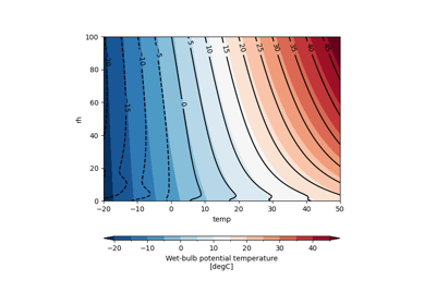
- easyclimate.physics.calc_wet_bulb_potential_temperature_iteration(temperature_data: xarray.DataArray, relative_humidity_data: xarray.DataArray, pressure_data: xarray.DataArray, temperature_data_units: Literal['celsius', 'kelvin', 'fahrenheit', 'degC', 'degK'], relative_humidity_data_units: Literal['%', 'dimensionless'], pressure_data_units: Literal['hPa', 'Pa', 'mbar'], A: float = 0.000662, tolerance: float = 0.01, max_iter: int = 100, method: Literal['easyclimate-backend', 'easyclimate-rust'] = 'easyclimate-rust') xarray.DataArray
Calculate wet-bulb potential temperature (\(\theta_w\)).
The iterative formula for wet-bulb temperature
\[e = e_{tw} - AP(t-t_{w})\]\(e\) is the water vapor pressure
\(e_{tw}\) is the saturation water vapor pressure over a pure flat ice surface at wet-bulb temperature \(t_w\) (when the wet-bulb thermometer is frozen, this becomes the saturation vapor pressure over a pure flat ice surface)
\(A\) is the psychrometer constant
\(P\) is the sea-level pressure
\(t\) is the dry-bulb temperature
\(t_w\) is the wet-bulb temperature
Wet-bulb potential temperature (\(\theta_w\)) is defined as the temperature that an air parcel would have if it were first brought to saturation at its ambient pressure (i.e., cooled to the wet-bulb temperature, \(T_w\)), and then brought dry-adiabatically to a reference pressure, conventionally (\(p_0 = 1000 \mathrm{hPa}\)).
This quantity is therefore obtained from two steps:
Compute the wet-bulb temperature (\(T_w\)) at the parcel’s pressure (\(p\));
Apply the dry-adiabatic (Poisson) transformation from (\(p\)) to (\(p_0\)).
Under this definition, once (\(T_w\)) is known, (\(\theta_w\)) follows directly as
\[\theta_w = (T_w + 273.15) ( \frac{p_0}{p}) ^{\kappa} - 273.15\]where \(\kappa = \frac{R_d}{c_p} \approx 0.2854\), and \(p_0 = 1000 \mathrm{hPa}\).
This formulation makes clear that the iterative/nonlinear part of the calculation is confined to determining (\(T_w\)); the mapping from (\(T_w\)) to (\(\theta_w\)) is purely algebraic via the dry-adiabatic relation.
Parameters
- temperature_data:
xarray.DataArray. Atmospheric temperature.
- relative_humidity_data:
xarray.DataArray. The relative humidity.
- pressure_data:
xarray.DataArray. The pressure data set.
- temperature_data_units:
str. The unit corresponding to temperature_data value. Optional values are celsius, kelvin, fahrenheit.
- relative_humidity_data_units:
str. The unit corresponding to vapor_pressure_data value. Optional values are
%,dimensionless.- pressure_data_units:
str. The unit corresponding to pressure_data value. Optional values are hPa, Pa, mbar.
- A:
float. Psychrometer coefficients.
Psychrometer Type and Ventilation Rate
Wet Bulb Unfrozen (10^-3/°C^-1)
Wet Bulb Frozen (10^-3/°C^-1)
Ventilated Psychrometer (2.5 m/s)
0.662
0.584
Spherical Psychrometer (0.4 m/s)
0.857
0.756
Cylindrical Psychrometer (0.4 m/s)
0.815
0.719
Chinese Spherical Psychrometer (0.8 m/s)
0.7949
0.7949
- tolerance:
float. Minimum acceptable deviation of the iterated value from the true value.
- max_iter:
int. Maximum number of iterations.
- method{“easyclimate-backend”,”easyclimate-rust”}
Backend implementation.
Notes
\(\theta_w\) is obtained by first computing the wet-bulb temperature (Tw) and then reducing it dry-adiabatically to 1000 hPa.
- easyclimate.physics.calc_wet_bulb_potential_temperature_davies_jones2008(pressure_data: xarray.DataArray, temperature_data: xarray.DataArray, dewpoint_data: xarray.DataArray, pressure_data_units: Literal['hPa', 'Pa', 'mbar'], temperature_data_units: Literal['celsius', 'kelvin', 'fahrenheit'], dewpoint_data_units: Literal['celsius', 'kelvin', 'fahrenheit']) xarray.DataArray
Calculate wet-bulb potential temperature using Robert Davies-Jones (2008) approximation.
Parameters
- pressure_data:
xarray.DataArray. The pressure data set.
- temperature_data:
xarray.DataArray. Atmospheric temperature.
- dewpoint_data:
xarray.DataArray. The dewpoint temperature.
- pressure_data_units:
str. The unit corresponding to pressure_data value. Optional values are hPa, Pa, mbar.
- temperature_data_units:
str. The unit corresponding to temperature_data value. Optional values are celsius, kelvin, fahrenheit.
- dewpoint_data_units:
str. The unit corresponding to dewpoint_data value. Optional values are celsius, kelvin, fahrenheit.
Returns
- tw:
xarray.DataArray( \(\mathrm{K}\) ) Wet-bulb temperature
See also
Davies-Jones, R. (2008). An Efficient and Accurate Method for Computing the Wet-Bulb Temperature along Pseudoadiabats. Monthly Weather Review, 136(7), 2764-2785. https://doi.org/10.1175/2007MWR2224.1
Knox, J. A., Nevius, D. S., & Knox, P. N. (2017). Two Simple and Accurate Approximations for Wet-Bulb Temperature in Moist Conditions, with Forecasting Applications. Bulletin of the American Meteorological Society, 98(9), 1897-1906. https://doi.org/10.1175/BAMS-D-16-0246.1
- pressure_data:
- easyclimate.physics.calc_wet_bulb_temperature_stull2011(temperature_data: xarray.DataArray, relative_humidity_data: xarray.DataArray, temperature_data_units: Literal['celsius', 'kelvin', 'fahrenheit'], relative_humidity_data_units: Literal['%', 'dimensionless']) xarray.DataArray
Calculate wet-bulb temperature using Stull (2011) empirical formula.
\[T_{w} =T\operatorname{atan}[0.151977(\mathrm{RH} \% +8.313659)^{1/2}]+\operatorname{atan}(T+\mathrm{RH}\%)-\operatorname{atan}(\mathrm{RH} \% -1.676331) +0.00391838(\mathrm{RH}\%)^{3/2}\operatorname{atan}(0.023101\mathrm{RH}\%)-4.686035.\]Tip
This methodology was not valid for ambient conditions with low values of \(T_a\) (dry-bulb temperature; i.e., <10°C), and/or with low values of RH (5% < RH < 10%). The Stull methodology was also only valid at sea level.
Parameters
- temperature_data:
xarray.DataArray. Atmospheric temperature.
- relative_humidity_data:
xarray.DataArray. The relative humidity.
- temperature_data_units:
str. The unit corresponding to temperature_data value. Optional values are celsius, kelvin, fahrenheit.
- relative_humidity_data_units:
str. The unit corresponding to vapor_pressure_data value. Optional values are
%,dimensionless.
Returns
- tw:
xarray.DataArray( \(\mathrm{K}\) ) Wet-bulb temperature
See also
Stull, R. (2011). Wet-Bulb Temperature from Relative Humidity and Air Temperature. Journal of Applied Meteorology and Climatology, 50(11), 2267-2269. https://doi.org/10.1175/JAMC-D-11-0143.1
Stull, R. (2011): Meteorology for Scientists and Engineers. 3rd ed. Discount Textbooks, 924 pp. [Available online at https://www.eoas.ubc.ca/books/Practical_Meteorology/, https://www.eoas.ubc.ca/courses/atsc201/MSE3.html]
Knox, J. A., Nevius, D. S., & Knox, P. N. (2017). Two Simple and Accurate Approximations for Wet-Bulb Temperature in Moist Conditions, with Forecasting Applications. Bulletin of the American Meteorological Society, 98(9), 1897-1906. https://doi.org/10.1175/BAMS-D-16-0246.1
- temperature_data:
- easyclimate.physics.calc_wet_bulb_temperature_sadeghi2013(temperature_data: xarray.DataArray, height_data: xarray.DataArray, relative_humidity_data: xarray.DataArray, temperature_data_units: Literal['celsius', 'kelvin', 'fahrenheit'], height_data_units: Literal['m', 'km'], relative_humidity_data_units: Literal['%', 'dimensionless']) xarray.DataArray
Calculate wet-bulb temperature using Sadeghi et. al (2011) empirical formula.
Parameters
- temperature_data:
xarray.DataArray. Atmospheric temperature.
- height_data:
xarray.DataArray. The elevation.
- relative_humidity_data:
xarray.DataArray. The relative humidity.
- temperature_data_units:
str. The unit corresponding to temperature_data value. Optional values are celsius, kelvin, fahrenheit.
- height_data_units:
str. The unit corresponding to height_data value. Optional values are m, km.
- relative_humidity_data_units:
str. The unit corresponding to vapor_pressure_data value. Optional values are
%,dimensionless.
Returns
- tw:
xarray.DataArray( \(\mathrm{degC}\) ) Wet-bulb temperature
See also
Sadeghi, S., Peters, T. R., Cobos, D. R., Loescher, H. W., & Campbell, C. S. (2013). Direct Calculation of Thermodynamic Wet-Bulb Temperature as a Function of Pressure and Elevation. Journal of Atmospheric and Oceanic Technology, 30(8), 1757-1765. https://doi.org/10.1175/JTECH-D-12-00191.1
- temperature_data:
- easyclimate.physics.calc_equivalent_potential_temperature(pressure_data: xarray.DataArray, temperature_data: xarray.DataArray, dewpoint_data: xarray.DataArray, pressure_data_units: Literal['hPa', 'Pa'], temperature_data_units: Literal['celsius', 'kelvin', 'fahrenheit'], dewpoint_data_units: Literal['celsius', 'kelvin', 'fahrenheit']) xarray.DataArray
Calculate equivalent potential temperature using Bolton (1980) approximation.
Parameters
- pressure_data:
xarray.DataArray. The pressure data set.
- temperature_data:
xarray.DataArray. Atmospheric temperature.
- dewpoint_data:
xarray.DataArray. The dew point temperature.
- pressure_data_units:
str. The unit corresponding to pressure_data value. Optional values are hPa, Pa.
- temperature_data_units:
str. The unit corresponding to temperature_data value. Optional values are celsius, kelvin, fahrenheit.
- dewpoint_data_units:
str. The unit corresponding to dewpoint_data value. Optional values are celsius, kelvin, fahrenheit.
Returns
- Equivalent potential temperature ( \(\mathrm{K}\) ).
See also
Bolton, D. (1980). The Computation of Equivalent Potential Temperature. Monthly Weather Review, 108(7), 1046-1053. https://journals.ametsoc.org/view/journals/mwre/108/7/1520-0493_1980_108_1046_tcoept_2_0_co_2.xml
- pressure_data:
- easyclimate.physics.calc_equivalent_potential_temperature_davies_jones2009(pressure_data: xarray.DataArray, temperature_data: xarray.DataArray, dewpoint_data: xarray.DataArray, pressure_data_units: Literal['hPa', 'Pa'], temperature_data_units: Literal['celsius', 'kelvin', 'fahrenheit'], dewpoint_data_units: Literal['celsius', 'kelvin', 'fahrenheit']) xarray.DataArray
Calculate equivalent potential temperature using Robert Davies-Jones (2009) approximation.
Parameters
- pressure_data:
xarray.DataArray. The pressure data set.
- temperature_data:
xarray.DataArray. Atmospheric temperature.
- dewpoint_data:
xarray.DataArray. The dew point temperature.
- pressure_data_units:
str. The unit corresponding to pressure_data value. Optional values are hPa, Pa.
- temperature_data_units:
str. The unit corresponding to temperature_data value. Optional values are celsius, kelvin, fahrenheit.
- dewpoint_data_units:
str. The unit corresponding to dewpoint_data value. Optional values are celsius, kelvin, fahrenheit.
Returns
- Equivalent potential temperature ( \(\mathrm{K}\) ).
See also
Davies-Jones, R. (2009). On Formulas for Equivalent Potential Temperature. Monthly Weather Review, 137(9), 3137-3148. https://doi.org/10.1175/2009MWR2774.1
- pressure_data:
- easyclimate.physics.calc_potential_temperature(temper_data: xarray.DataArray, pressure_data: xarray.DataArray, pressure_data_units: Literal['hPa', 'Pa', 'mbar'], kappa: float = 287 / 1005.7) xarray.DataArray
Calculate the potential temperature for dry air.
Uses the Poisson equation to calculation the potential temperature given pressure and temperature.
\[\theta = T \left( \frac{p_0}{p} \right) ^\kappa\]Parameters
- temper_data:
xarray.DataArray. Air temperature.
- pressure_data:
xarray.DataArray. The pressure data set.
- pressure_data_units:
str. The unit corresponding to pressure_data value. Optional values are hPa, Pa.
- kappa:
float, default: 287/1005.7. Poisson constant \(\kappa\).
Returns
- Potential temperature, units according to
temper_data.
Reference
Bolton, D. (1980). The Computation of Equivalent Potential Temperature. Monthly Weather Review, 108(7), 1046-1053. https://journals.ametsoc.org/view/journals/mwre/108/7/1520-0493_1980_108_1046_tcoept_2_0_co_2.xml
- temper_data:
- easyclimate.physics.calc_potential_temperature_vertical(temper_data: xarray.DataArray, vertical_dim: str, vertical_dim_units: Literal['hPa', 'Pa', 'mbar'], kappa: float = 287 / 1005.7) xarray.DataArray
Calculate the potential temperature for vertical variables.
Uses the Poisson equation to calculation the potential temperature given pressure and temperature.
\[\theta = T \left( \frac{p_0}{p} \right) ^\kappa\]Parameters
- temper_data:
xarray.DataArray. Air temperature.
- vertical_dim:
str. Vertical coordinate dimension name.
- vertical_dim_units:
str. The unit corresponding to the vertical p-coordinate value. Optional values are hPa, Pa, mbar.
- kappa:
float, default: 287/1005.7. Poisson constant \(\kappa\).
Returns
- Potential temperature, units according to
temper_data.
Reference
- temper_data:
- easyclimate.physics.calc_virtual_temperature(temper_data: xarray.DataArray, specific_humidity_data: xarray.DataArray, specific_humidity_data_units: Literal['kg/kg', 'g/g', 'g/kg'], epsilon: float = 0.608) xarray.DataArray
Calculate virtual temperature.
The virtual temperature (\(T_v\)) is the temperature at which dry air would have the same density as the moist air, at a given pressure. In other words, two air samples with the same virtual temperature have the same density, regardless of their actual temperature or relative humidity. The virtual temperature is always greater than the absolute air temperature.
\[T_v = T(1+ \epsilon q)\]where \(\epsilon = 0.608\) when the mixing ratio (specific humidity) \(q\) is expressed in \(\mathrm{g \cdot g^{-1}}\).
Parameters
- temper_data:
xarray.DataArray. Air temperature.
- specific_humidity_data:
xarray.DataArray. The absolute humidity data.
- specific_humidity_data_units:
str. The unit corresponding to specific_humidity value. Optional values are kg/kg, g/g, g/kg and so on.
- epsilon:
float. A constant.
Returns
- The virtual temperature, units according to
temper_data.
Reference
Doswell, C. A., and E. N. Rasmussen, 1994: The Effect of Neglecting the Virtual Temperature Correction on CAPE Calculations. Wea. Forecasting, 9, 625–629, https://journals.ametsoc.org/view/journals/wefo/9/4/1520-0434_1994_009_0625_teontv_2_0_co_2.xml
- temper_data:
- easyclimate.physics.calc_virtual_temperature_Hobbs2006(temper_data: xarray.DataArray, specific_humidity_data: xarray.DataArray, specific_humidity_data_units: Literal['kg/kg', 'g/g', 'g/kg'], epsilon: float = 0.6219569100577033) xarray.DataArray
Calculate virtual temperature.
The virtual temperature (\(T_v\)) is the temperature at which dry air would have the same density as the moist air, at a given pressure. In other words, two air samples with the same virtual temperature have the same density, regardless of their actual temperature or relative humidity. The virtual temperature is always greater than the absolute air temperature.
This calculation must be given an air parcel’s temperature and mixing ratio. The implementation uses the formula outlined in [Hobbs2006] pg.67 & 80.
\[T_v = T \frac{\text{q} + \epsilon}{\epsilon\,(1 + \text{q})}\]where \(\epsilon \approx 0.622\) when the mixing ratio (specific humidity) \(q\) is expressed in \(\mathrm{g \ g^{-1}}\).
Parameters
- temper_data:
xarray.DataArray. Air temperature.
- specific_humidity_data:
xarray.DataArray. The absolute humidity data.
- specific_humidity_data_units:
str. The unit corresponding to specific_humidity value. Optional values are kg/kg, g/g, g/kg and so on.
- epsilon:
float. The molecular weight ratio, which is molecular weight of the constituent gas to that assumed for air. Defaults to the ratio for water vapor to dry air. (\(\epsilon \approx 0.622\))
Returns
- The virtual temperature, units according to
temper_data.
Reference
Hobbs, P. V., and J. M. Wallace, 2006: Atmospheric Science: An Introductory Survey. 2nd ed. Academic Press, 504 pp. https://www.sciencedirect.com/book/9780127329512/atmospheric-science
Doswell, C. A., and E. N. Rasmussen, 1994: The Effect of Neglecting the Virtual Temperature Correction on CAPE Calculations. Wea. Forecasting, 9, 625–629, https://journals.ametsoc.org/view/journals/wefo/9/4/1520-0434_1994_009_0625_teontv_2_0_co_2.xml
- temper_data:
- easyclimate.physics.calc_lifting_condensation_level_bolton1980(temperature_data: xarray.DataArray, relative_humidity_data: xarray.DataArray, temperature_data_units: Literal['celsius', 'kelvin', 'fahrenheit'], relative_humidity_data_units: Literal['%', 'dimensionless']) xarray.DataArray
Calculate lifting condensation level using Bolton (1980) approximation.
\[T_L = \frac{1}{\frac{1}{T_K - 55} - \frac{\ln (U/100)}{2840}} + 55\]Parameters
- temperature_data:
xarray.DataArray. Atmospheric temperature.
- relative_humidity_data:
xarray.DataArray. The relative humidity.
- temperature_data_units:
str. The unit corresponding to temperature_data value. Optional values are
celsius,kelvin,fahrenheit.- relative_humidity_data_units:
str. The unit corresponding to vapor_pressure_data value. Optional values are
%,dimensionless.
Returns
- The lifting condensation level ( \(\mathrm{K}\) ).
See also
Bolton, D. (1980). The Computation of Equivalent Potential Temperature. Monthly Weather Review, 108(7), 1046-1053. https://journals.ametsoc.org/view/journals/mwre/108/7/1520-0493_1980_108_1046_tcoept_2_0_co_2.xml
- temperature_data:
- easyclimate.physics.calc_lifting_condensation_level_Bohren_Albrecht2023(pressure_data: xarray.DataArray, temperature_data: xarray.DataArray, dewpoint_data: xarray.DataArray, pressure_data_units: Literal['hPa', 'Pa', 'mbar'], temperature_data_units: Literal['celsius', 'kelvin', 'fahrenheit'], dewpoint_data_units: Literal['celsius', 'kelvin', 'fahrenheit']) xarray.Dataset
Calculate lifting condensation level using Bohren & Albrecht (2023) approximation.
According to formulation (6.32) in Bohren & Albrecht (2023),
\[T_{LCL}=\frac{1-AT_d}{1/T_d + B\ln(T/T_d)-A}\]Where
\[A=-\left(\frac{c_{pv}-c_{pw}}{l_r}-\frac{c_{pd}}{\epsilon l_v}\right),\quad B=\frac{c_{pd}}{\epsilon l_v}\]and
\[l_v=l_{vr} - (c_{pv}-c_{pw})T_r, \quad l_v(T_d)=l_r+(c_{pd} - c_{pw}) T_d\]Parameters
- pressure_data:
xarray.DataArray. The pressure data set.
- temperature_data:
xarray.DataArray. Atmospheric temperature.
- dewpoint_data:
xarray.DataArray. The dewpoint temperature.
- pressure_data_units:
str. The unit corresponding to pressure_data value. Optional values are hPa, Pa, mbar.
- temperature_data_units:
str. The unit corresponding to temperature_data value. Optional values are celsius, kelvin, fahrenheit.
- dewpoint_data_units:
str. The unit corresponding to dewpoint_data value. Optional values are celsius, kelvin, fahrenheit.
Returns
The lifting condensation level (
xarray.Dataset)p_lcl: lifting condensation level pressure ( \(\mathrm{hPa}\) ).
t_lcl: lifting condensation level temperature ( \(\mathrm{K}\) ).
See also
Bohren, C. F., and B. A. Albrecht, 2023: Atmospheric Thermodynamics Second Edition. Oxford University Press, 579 pp. Website: http://gen.lib.rus.ec/book/index.php?md5=AA3B25841BE3AEBA2628EF9961F58C52
- pressure_data:
- easyclimate.physics.calc_brunt_vaisala_frequency_atm(potential_temperature_data: xarray.DataArray, z_data: xarray.DataArray, vertical_dim: str, g: float = 9.8) xarray.DataArray
Calculation of the Brunt-väisälä frequency for the vertical atmosphere.
\[N = \left( \frac{g}{\theta} \frac{\mathrm{d}\theta}{\mathrm{d}z} \right)^\frac{1}{2}\]Parameters
- potential_temperature_data:
xarray.DataArray. Vertical atmospheric potential temperature.
- z_data:
xarray.DataArray( \(\mathrm{m}\) ). Vertical atmospheric geopotential height.
Attention
The unit of z_data should be meters, NOT \(\mathrm{m^2 \cdot s^2}\) which is the unit used in the representation of potential energy.
Returns
- Brunt-väisälä frequency, units according to
potential_temperature_data\(^{1/2}\).
Reference
- potential_temperature_data:
- easyclimate.physics.calc_static_stability(temper_data: xarray.DataArray, vertical_dim: str, vertical_dim_units: Literal['hPa', 'Pa', 'mbar']) xarray.DataArray
Calculate the static stability within a vertical profile.
\[\sigma = - T \frac{\partial \ln \theta}{\partial p}\]Parameters
- temper_data:
xarray.DataArray. Air temperature.
- vertical_dim:
str. Vertical coordinate dimension name.
- vertical_dim_units:
str. The unit corresponding to the vertical p-coordinate value. Optional values are hPa, Pa, mbar.
Returns
- Static stability, units according to
temper_data_units^2 vertical_dim_units^-1.
Reference
Howard B. Bluestein. (1992). Synoptic-Dynamic Meteorology in Midlatitudes: Principles of Kinematics and Dynamics, Vol. 1
- temper_data:
- easyclimate.physics.calc_enthalpy(temperature_data: xarray.DataArray, mixing_ratio_data: xarray.DataArray, temperature_data_units: Literal['celsius', 'kelvin', 'fahrenheit'], mixing_ratio_data_units: Literal['kg/kg', 'g/g', 'g/kg']) xarray.DataArray
Calculate atmospheric enthalpy from temperature and humidity mixing ratio.
Enthalpy is a thermodynamic quantity equivalent to the internal energy plus the energy the system exerts on its surroundings. The enthalpy is a constant pressure function. As such, it includes the work term for expansion against the atmosphere.
\[T \cdot (1.01 + 0.00189 \cdot W) + 2.5 \cdot W\]where the unit of \(T\) (atmospheric temperature) is
degC, and \(W\) (mixing ratio) isg/kg.Parameters
- temperature_data:
xarray.DataArray. Atmospheric temperature.
- mixing_ratio_data:
xarray.DataArray. The mixing ratio of a gas.
- temperature_data_units:
str. The unit corresponding to temperature_data value. Optional values are celsius, kelvin, fahrenheit.
- mixing_ratio_data_units:
str. The unit corresponding to
mixing_ratio_datavalue. Optional values are \(\mathrm{kg/kg}\), \(\mathrm{g/g}\), \(\mathrm{g/kg}\) and so on.
Returns
- Atmospheric enthalpy ( \(\mathrm{kJ/kg}\) ).
- temperature_data:
- easyclimate.physics.calc_latent_heat_water(temperature_data, temperature_data_units: Literal['celsius', 'kelvin', 'fahrenheit'], latent_heat_type: Literal['evaporation_condensation', 'melting_freezing', 'sublimation_deposition']) xarray.DataArray
Estimate latent heat flux for water: evaporization (condensation), melting (freezing) or sublimation (deposition).
Tip
This function returns the latent heat of
evaporation/condensation
melting/freezing
sublimation/deposition
for water. The latent heatis a function of temperature t. The formulas are polynomial approximations to the values in Table 92, p. 343 of the Smithsonian Meteorological Tables, Sixth Revised Edition, 1963 by Roland List. The approximations were developed by Eric Smith at Colorado State University.
Source: Thomas W. Schlatter and Donald V. Baker: PROFS Program Office, NOAA Environmental Research Laboratories, Boulder, Colorado.
Parameters
- temperature_data:
xarray.DataArray. Atmospheric temperature.
- temperature_data_units:
str. The unit corresponding to temperature_data value. Optional values are
celsius,kelvin,fahrenheit.- latent_heat_type:
str. The type of latent heat to estimate. Optional values are
evaporation_condensation,melting_freezing,sublimation_deposition.
Returns
- Latent heat flux for water ( \(\mathrm{J/kg}\) ).
- easyclimate.physics.calc_relative_angular_momentum(zonal_wind_speed_data: xarray.DataArray, vertical_dim: str, vertical_dim_units: Literal['hPa', 'Pa', 'mbar'], lon_dim: str = 'lon', lat_dim: str = 'lat', weights=None)
Calculate atmospheric relative angular momentum.
Parameters
- zonal_wind_speed_data
xarray.DataArray( \(\mathrm{m/s}\) ) Zonal wind component with the least similar dimensions
(vertical_dim, lon_dim, lat_dim)- vertical_dim:
str. Vertical coordinate dimension name.
- vertical_dim_units:
str. The unit corresponding to the vertical p-coordinate value. Optional values are
hPa,Pa,mbar.- lon_dim:
str, default:lon. Longitude coordinate dimension name. By default extracting is applied over the
londimension.- lat_dim:
str, default:lat. Latitude coordinate dimension name. By default extracting is applied over the
latdimension.- weights
xarray.DataArray, optional Weights for each latitude, same dimension as lat. If None, computed as \(\cos(lat)*\mathrm{d}lat\) with the values of
latitudespacing.
Returns
- aam
xarray.DataArray( \(\mathrm{kg} \cdot \mathrm{m^2/s}\) ) Atmospheric angular momentum.
- zonal_wind_speed_data
- easyclimate.physics.transfer_mixing_ratio_2_specific_humidity(mixing_ratio_data: xarray.DataArray, mixing_ratio_data_units: Literal['kg/kg', 'g/g', 'g/kg']) xarray.DataArray
Calculate the specific humidity from mixing ratio.
Parameters
- mixing_ratio_data:
xarray.DataArray. The mixing ratio of a gas.
- mixing_ratio_data_units:
str. The unit corresponding to
mixing_ratio_datavalue. Optional values are \(\mathrm{kg/kg}\), \(\mathrm{g/g}\), \(\mathrm{g/kg}\) and so on.
Returns
- The specific humidity, dimensionless (e.g. \(\mathrm{kg/kg}\), \(\mathrm{g/g}\)).
- mixing_ratio_data:
- easyclimate.physics.transfer_specific_humidity_2_mixing_ratio(specific_humidity_data: xarray.DataArray, specific_humidity_data_units: Literal['kg/kg', 'g/g', 'g/kg']) xarray.DataArray
Calculate the mixing ratio from specific humidity.
Parameters
- specific_humidity_data:
xarray.DataArray. The Specific humidity of air.
- specific_humidity_data_units:
str. The unit corresponding to specific_humidity value. Optional values are \(\mathrm{kg/kg}\), \(\mathrm{g/g}\), \(\mathrm{g/kg}\) and so on.
Returns
- The mixing ratio, dimensionless (e.g. \(\mathrm{kg/kg}\), \(\mathrm{g/g}\)).
- specific_humidity_data:
- easyclimate.physics.transfer_dewpoint_2_specific_humidity(dewpoint_data: xarray.DataArray, pressure_data: xarray.DataArray, dewpoint_data_units: Literal['celsius', 'kelvin', 'fahrenheit'], pressure_data_units: Literal['hPa', 'Pa', 'mbar']) xarray.DataArray
Calculate the specific humidity from the dew point temperature and pressure.
Parameters
- dewpoint_data:
xarray.DataArray. The dew point temperature.
- pressure_data:
xarray.DataArray. The pressure data set.
- dewpoint_data_units:
str. The unit corresponding to dewpoint_data value. Optional values are celsius, kelvin, fahrenheit.
- pressure_data_units:
str. The unit corresponding to pressure_data value. Optional values are hPa, Pa.
Returns
- The specific humidity, dimensionless (e.g. \(\mathrm{kg/kg}\), \(\mathrm{g/g}\)).
- dewpoint_data:
- easyclimate.physics.transfer_dewpoint_2_mixing_ratio(dewpoint_data: xarray.DataArray, pressure_data: xarray.DataArray, dewpoint_data_units: Literal['celsius', 'kelvin', 'fahrenheit'], pressure_data_units: Literal['hPa', 'Pa', 'mbar'])
Calculate the mixing ratio from the dew point temperature and pressure.
Parameters
- dewpoint_data:
xarray.DataArray. The dew point temperature.
- pressure_data:
xarray.DataArray. The pressure data set.
- dewpoint_data_units:
str. The unit corresponding to dewpoint_data value. Optional values are celsius, kelvin, fahrenheit.
- pressure_data_units:
str. The unit corresponding to pressure_data value. Optional values are hPa, Pa.
Returns
- The mixing ratio, dimensionless (e.g. \(\mathrm{kg/kg}\), \(\mathrm{g/g}\)).
- dewpoint_data:
- easyclimate.physics.transfer_specific_humidity_2_dewpoint(specific_humidity_data: xarray.DataArray, pressure_data: xarray.DataArray, specific_humidity_data_units: Literal['kg/kg', 'g/g', 'g/kg'], pressure_data_units: Literal['hPa', 'Pa', 'mbar'], epsilon: float = 0.6219569100577033) xarray.DataArray
Calculate the dew point temperature from specific humidity and pressure.
Parameters
- specific_humidity_data:
xarray.DataArray. The absolute humidity data.
- pressure_data:
xarray.DataArray. The pressure data set.
- specific_humidity_data_units:
str. The unit corresponding to specific_humidity value. Optional values are \(\mathrm{kg/kg}\), \(\mathrm{g/g}\), \(\mathrm{g/kg}\) and so on.
- pressure_data_units:
str. The unit corresponding to pressure_data value. Optional values are hPa, Pa.
- epsilon:
float. The molecular weight ratio, which is molecular weight of the constituent gas to that assumed for air. Defaults to the ratio for water vapor to dry air. (\(\epsilon \approx 0.622\))
Returns
- The dew point temperature ( \(\mathrm{degC}\) ).
- specific_humidity_data:
- easyclimate.physics.transfer_dewpoint_2_relative_humidity(temperature_data: xarray.DataArray, dewpoint_data: xarray.DataArray, temperature_data_units: Literal['celsius', 'kelvin', 'fahrenheit'], dewpoint_data_units: Literal['celsius', 'kelvin', 'fahrenheit']) xarray.DataArray
Calculate the relative humidity from dew point temperature.
Uses temperature and dew point temperature to calculate relative humidity as the ratio of vapor pressure to saturation vapor pressures.
Parameters
- temperature_data:
xarray.DataArray. Atmospheric temperature.
- dewpoint_data:
xarray.DataArray. The dew point temperature.
- temperature_data_units:
str. The unit corresponding to temperature_data value. Optional values are celsius, kelvin, fahrenheit.
- dewpoint_data_units:
str. The unit corresponding to dewpoint_data value. Optional values are celsius, kelvin, fahrenheit.
Returns
- The relative humidity, dimensionless.
- temperature_data:
- easyclimate.physics.transfer_mixing_ratio_2_relative_humidity(pressure_data: xarray.DataArray, temperature_data: xarray.DataArray, mixing_ratio_data: xarray.DataArray, pressure_data_units: Literal['hPa', 'Pa', 'mbar'], temperature_data_units: Literal['celsius', 'kelvin', 'fahrenheit'], mixing_ratio_data_units: Literal['kg/kg', 'g/g', 'g/kg'], epsilon: float = 0.6219569100577033) xarray.DataArray
Calculate the relative humidity from mixing ratio, temperature, and pressure.
Parameters
- pressure_data:
xarray.DataArray. The pressure data set.
- temperature_data:
xarray.DataArray. Atmospheric temperature.
- mixing_ratio_data:
xarray.DataArray. The mixing ratio of a gas.
- pressure_data_units:
str. The unit corresponding to pressure_data value. Optional values are hPa, Pa.
- temperature_data_units:
str. The unit corresponding to temperature_data value. Optional values are celsius, kelvin, fahrenheit.
- mixing_ratio_data_units:
str. The unit corresponding to
mixing_ratio_datavalue. Optional values are \(\mathrm{kg/kg}\), \(\mathrm{g/g}\), \(\mathrm{g/kg}\) and so on.- epsilon:
float. The molecular weight ratio, which is molecular weight of the constituent gas to that assumed for air. Defaults to the ratio for water vapor to dry air. (\(\epsilon \approx 0.622\))
Returns
- The relative humidity, dimensionless.
- pressure_data:
- easyclimate.physics.transfer_specific_humidity_2_relative_humidity(pressure_data: xarray.DataArray, temperature_data: xarray.DataArray, specific_humidity_data: xarray.DataArray, pressure_data_units: Literal['hPa', 'Pa', 'mbar'], temperature_data_units: Literal['celsius', 'kelvin', 'fahrenheit'], specific_humidity_data_units: Literal['kg/kg', 'g/g', 'g/kg']) xarray.DataArray
Calculate the relative humidity from specific humidity, temperature, and pressure.
Parameters
- pressure_data:
xarray.DataArray. The pressure data set.
- temperature_data:
xarray.DataArray. Atmospheric temperature.
- specific_humidity_data:
xarray.DataArray. The absolute humidity data.
- pressure_data_units:
str. The unit corresponding to pressure_data value. Optional values are hPa, Pa.
- temperature_data_units:
str. The unit corresponding to temperature_data value. Optional values are celsius, kelvin, fahrenheit.
- specific_humidity_data_units:
str. The unit corresponding to specific_humidity value. Optional values are \(\mathrm{kg/kg}\), \(\mathrm{g/g}\), \(\mathrm{g/kg}\) and so on.
Returns
- The relative humidity, dimensionless.
- pressure_data:
- easyclimate.physics.transfer_relative_humidity_2_dewpoint(relative_humidity_data: xarray.DataArray, temperature_data: xarray.DataArray, relative_humidity_data_units: Literal['%', 'dimensionless'], temperature_data_units: Literal['celsius', 'kelvin', 'fahrenheit']) xarray.DataArray
Calculate dew point temperature from temperature and relative humidity.
The dew point temperature given temperature and relative humidity using the equations from John Dutton’s “Ceaseless Wind” (pp 273-274). Missing values are ignored.
The dew point temperature \(T_d\) (in Kelvin) is calculated from temperature \(T\) and relative humidity \(RH\) using the formula:
\[T_d = \frac{T \cdot L}{L - T \cdot \ln(RH/100)}, \quad \text{where} \quad L = \frac{597.3 - 0.57(T - 273.0)}{GCX} \quad \text{and} \quad GCX = \frac{461.5}{4186}.\]Parameters
- relative_humidity_data:
xarray.DataArray. The relative humidity.
- temperature_data:
xarray.DataArray. Atmospheric temperature.
- relative_humidity_data_units:
str. The unit corresponding to vapor_pressure_data value. Optional values are
%,dimensionless.- temperature_data_units:
str. The unit corresponding to
temperature_datavalue. Optional values arecelsius,kelvin,fahrenheit.
Returns
- dewpoint
xarray.DataArray( \(\mathrm{K}\) ) Dew point temperature.
Reference
Dutton, J. A. (1976). The Ceaseless Wind: An introduction to the theory of atmospheric motion. McGraw-Hill, Inc. https://libgen.li/file.php?md5=7154c67714c7aee56152cfda528e2080
- relative_humidity_data: