MPAS Cell-centered quiver plots

This example shows how to draw MPAS cell-centered vector winds with easyclimate.plot.mpas.plot_cell_quiver.

The input zonal and meridional components are one-dimensional variables on nCells after selecting a time and vertical level. The plotting helper thins the vectors in longitude-latitude bins before drawing them.

import xarray as xr
import numpy as np
import cartopy.crs as ccrs
import matplotlib.pyplot as plt
import easyclimate as ecl

from easyclimate.plot.mpas import plot_cell_quiver

Open MPAS output and select a horizontal wind field on cell centers.

data = ecl.open_tutorial_dataset("mpas_JWwave_T10_nVertLevels10")
U = data.uReconstructZonal
V = data.uReconstructMeridional

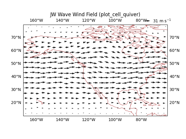
Draw a regional quiver plot. thin_method="nearest_center" keeps the vector closest to each bin center, which preserves sampled MPAS values.

fig, ax = plt.subplots(subplot_kw= {"projection": ccrs.PlateCarree(-120)})

cq = plot_cell_quiver(
    data,
    U,
    V,

    lon_min=190,
    lon_max=-60,
    lat_min=10,
    lat_max=80,

    nx_bins=25,
    ny_bins=18,

    thin_method="nearest_center",
    scale=900,
    width = 0.004,
    headaxislength = 5,
)

ax.set_title("JW Wave Wind Field (plot_cell_quiver)")
ax.coastlines(resolution="110m", linewidth=0.6, color = "brown")
ax.gridlines(draw_labels=True, alpha = 0)

<cartopy.mpl.gridliner.Gridliner object at 0x7a87977e0fb0>

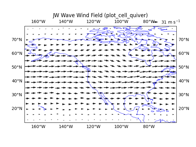
thin_method="mean" averages vectors within each bin. This is useful when a smoother regional wind depiction is desired.

fig, ax = plt.subplots(subplot_kw= {"projection": ccrs.PlateCarree(-120)})

cq = plot_cell_quiver(
    data,
    U,
    V,

    lon_min=190,
    lon_max=-60,
    lat_min=10,
    lat_max=80,

    nx_bins=25,
    ny_bins=18,

    thin_method="mean",
    scale=900,
    width = 0.004,
    headaxislength = 5,
)

ax.set_title("JW Wave Wind Field (plot_cell_quiver)")
ax.coastlines(resolution="110m", linewidth=0.6, color = "b")
ax.gridlines(draw_labels=True, alpha = 0)

<cartopy.mpl.gridliner.Gridliner object at 0x7a8799de5f40>

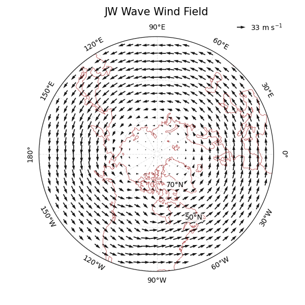
For polar projections, regrid_shape lets Cartopy place vectors on the map projection grid before drawing.

fig, ax = plt.subplots(
    figsize = (6, 6),
    subplot_kw={"projection": ccrs.NorthPolarStereo(central_longitude=-90)}
)

ax.coastlines(color="brown", linewidths=0.5)

cq = plot_cell_quiver(
    data,
    U,
    V,

    lon_min=0,
    lon_max=360,
    lat_min=30,
    lat_max=90,

    nx_bins=80,
    ny_bins=18,

    thin_method="nearest_center",
    title="",

    scale=900,
    regrid_shape = 30,
    width = 0.004,
    headaxislength = 5,
)

gl, meta = ecl.plot.draw_polar_basemap(
    ax = ax,
    lon_step=30,
    lat_step=20,
    lat_range=[30, 90],
    draw_labels=True,
    gridlines_kwargs={"color": "grey", "alpha": 0.2, "linestyle": "--"},
    lat_label_lon=-60
)

ecl.plot.set_polar_title("JW Wave Wind Field", meta, size = 15)

Text(0.5, 1.0831890201695809, 'JW Wave Wind Field')