MPAS Cell-centered contour plots

This example demonstrates filled and line contours for MPAS cell-centered scalar fields.

easyclimate.plot.mpas.plot_cell_contourf draws filled contours from values located on nCells. The companion easyclimate.plot.mpas.plot_cell_contour draws contour lines using the same MPAS cell coordinates.

import xarray as xr
import numpy as np
import cartopy.crs as ccrs
import matplotlib.pyplot as plt
import easyclimate as ecl

from easyclimate.plot.mpas import plot_cell_contourf, plot_cell_contour

Open a sample MPAS output file. The divergence variable is defined at MPAS cell centers, so one time and vertical level are selected before plotting.

data = ecl.open_tutorial_dataset("mpas_JWwave_T10_nVertLevels10")
data

<xarray.Dataset> Size: 6MB
Dimensions:                 (nCells: 40962, nVertices: 81920, maxEdges: 10,
                             nEdges: 122880, TWO: 2, vertexDegree: 3)
Coordinates:
  * nCells                  (nCells) int64 328kB 0 1 2 3 ... 40959 40960 40961
    Time                    int64 8B ...
    nVertLevels             int64 8B ...
Dimensions without coordinates: nVertices, maxEdges, nEdges, TWO, vertexDegree
Data variables:
    uReconstructZonal       (nCells) float32 164kB ...
    uReconstructMeridional  (nCells) float32 164kB ...
    vorticity               (nVertices) float32 328kB ...
    divergence              (nCells) float32 164kB ...
    lonCell                 (nCells) float32 164kB ...
    latCell                 (nCells) float32 164kB ...
    lonVertex               (nVertices) float32 328kB ...
    latVertex               (nVertices) float32 328kB ...
    verticesOnCell          (nCells, maxEdges) int32 2MB ...
    nEdgesOnCell            (nCells) int32 164kB ...
    verticesOnEdge          (nEdges, TWO) int32 983kB ...
    cellsOnVertex           (nVertices, vertexDegree) int32 983kB ...
Attributes: (12/180)
    model_name:                             mpas
    core_name:                              atmosphere
    version:                                8.4.0
    source:                                 MPAS
    Conventions:                            MPAS
    git_version:                            v8.4.0
    ...                                     ...
    config_noahmp_iopt_crop:                0
    config_noahmp_iopt_irr:                 0
    config_noahmp_iopt_irrm:                0
    config_noahmp_iopt_infdv:               1
    config_noahmp_iopt_tdrn:                0
    file_id:                                m02zbs7ciw

xarray.Dataset

• Dimensions:
  • nCells: 40962
  • nVertices: 81920
  • maxEdges: 10
  • nEdges: 122880
  • TWO: 2
  • vertexDegree: 3
• Coordinates: (3)
  • nCells
    (nCells)
    int64
    0 1 2 3 ... 40958 40959 40960 40961

    array([    0,     1,     2, ..., 40959, 40960, 40961], shape=(40962,))

  • Time
    ()
    int64
    ...

    [1 values with dtype=int64]

  • nVertLevels
    ()
    int64
    ...

    [1 values with dtype=int64]

• Data variables: (12)
  • uReconstructZonal
    (nCells)
    float32
    ...

    units :

    m s^{-1}

    long_name :

    Zonal component of reconstructed horizontal velocity at cell centers

    [40962 values with dtype=float32]

  • uReconstructMeridional
    (nCells)
    float32
    ...

    units :

    m s^{-1}

    long_name :

    Meridional component of reconstructed horizontal velocity at cell centers

    [40962 values with dtype=float32]

  • vorticity
    (nVertices)
    float32
    ...

    units :

    s^{-1}

    long_name :

    Relative vorticity at vertices

    [81920 values with dtype=float32]

  • divergence
    (nCells)
    float32
    ...

    units :

    s^{-1}

    long_name :

    Horizontal velocity divergence at cell center

    [40962 values with dtype=float32]

  • lonCell
    (nCells)
    float32
    ...

    units :

    rad

    long_name :

    Longitude of cells

    [40962 values with dtype=float32]

  • latCell
    (nCells)
    float32
    ...

    units :

    rad

    long_name :

    Latitude of cells

    [40962 values with dtype=float32]

  • lonVertex
    (nVertices)
    float32
    ...

    units :

    rad

    long_name :

    Longitude of vertices

    [81920 values with dtype=float32]

  • latVertex
    (nVertices)
    float32
    ...

    units :

    rad

    long_name :

    Latitude of vertices

    [81920 values with dtype=float32]

  • verticesOnCell
    (nCells, maxEdges)
    int32
    ...

    units :

    -

    long_name :

    IDs of vertices (corner points) of a cell

    [409620 values with dtype=int32]

  • nEdgesOnCell
    (nCells)
    int32
    ...

    units :

    -

    long_name :

    Number of edges forming the boundary of a cell

    [40962 values with dtype=int32]

  • verticesOnEdge
    (nEdges, TWO)
    int32
    ...

    units :

    -

    long_name :

    IDs of the two vertex endpoints of an edge

    [245760 values with dtype=int32]

  • cellsOnVertex
    (nVertices, vertexDegree)
    int32
    ...

    units :

    -

    long_name :

    IDs of the cells that meet at a vertex

    [245760 values with dtype=int32]

• Attributes: (180)

  model_name :

  mpas

  core_name :

  atmosphere

  version :

  8.4.0

  source :

  MPAS

  Conventions :

  MPAS

  git_version :

  v8.4.0

  on_a_sphere :

  YES

  sphere_radius :

  6.371229e+06

  is_periodic :

  NO

  x_period :

  0.0

  y_period :

  0.0

  history :

  mpirun -n 2 ./atmosphere_model

  parent_id :

  obz1o02d1d

  mesh_spec :

  0.0

  config_time_integration :

  SRK3

  config_time_integration_order :

  2

  config_dt :

  450.0

  config_calendar_type :

  gregorian

  config_start_time :

  0000-01-01_00:00:00

  config_stop_time :

  none

  config_run_duration :

  16_00:00:00

  config_split_dynamics_transport :

  NO

  config_number_of_sub_steps :

  6

  config_dynamics_split_steps :

  1

  config_h_mom_eddy_visc2 :

  0.0

  config_h_mom_eddy_visc4 :

  0.0

  config_v_mom_eddy_visc2 :

  0.0

  config_h_theta_eddy_visc2 :

  0.0

  config_h_theta_eddy_visc4 :

  0.0

  config_v_theta_eddy_visc2 :

  0.0

  config_horiz_mixing :

  2d_smagorinsky

  config_les_model :

  none

  config_les_surface :

  none

  config_surface_heat_flux :

  0.0

  config_surface_moisture_flux :

  0.0

  config_surface_drag_coefficient :

  0.0

  config_len_disp :

  120000.0

  config_visc4_2dsmag :

  0.05

  config_mix_scalars :

  NO

  config_del4u_div_factor :

  10.0

  config_w_adv_order :

  3

  config_theta_adv_order :

  3

  config_scalar_adv_order :

  3

  config_u_vadv_order :

  3

  config_w_vadv_order :

  3

  config_theta_vadv_order :

  3

  config_scalar_vadv_order :

  3

  config_scalar_advection :

  NO

  config_positive_definite :

  NO

  config_monotonic :

  NO

  config_coef_3rd_order :

  1.0

  config_smagorinsky_coef :

  0.125

  config_mix_full :

  YES

  config_epssm :

  0.1

  config_smdiv :

  0.1

  config_apvm_upwinding :

  0.5

  config_h_ScaleWithMesh :

  YES

  config_num_halos :

  2

  config_relax_zone_divdamp_coef :

  6.0

  config_zd :

  22000.0

  config_xnutr :

  0.0

  config_mpas_cam_coef :

  0.0

  config_number_cam_damping_levels :

  4

  config_rayleigh_damp_u :

  NO

  config_rayleigh_damp_u_timescale_days :

  5.0

  config_number_rayleigh_damp_u_levels :

  6

  config_epssm_minimum :

  0.1

  config_epssm_maximum :

  0.5

  config_epssm_transition_bottom_z :

  30000.0

  config_epssm_transition_top_z :

  50000.0

  config_apply_lbcs :

  NO

  config_restart_timestamp_name :

  restart_timestamp

  config_pio_num_iotasks :

  0

  config_pio_stride :

  1

  config_block_decomp_file_prefix :

  x1.40962.graph.info.part.

  config_number_of_blocks :

  0

  config_explicit_proc_decomp :

  NO

  config_proc_decomp_file_prefix :

  graph.info.part.

  config_do_restart :

  NO

  config_do_DAcycling :

  NO

  config_print_global_minmax_vel :

  YES

  config_print_detailed_minmax_vel :

  NO

  config_print_global_minmax_sca :

  NO

  config_IAU_option :

  off

  config_IAU_window_length_s :

  21600.0

  config_jedi_da :

  NO

  config_halo_exch_method :

  mpas_halo

  config_gpu_aware_mpi :

  NO

  input_soil_data :

  STAS

  input_soil_temperature_lag :

  140

  num_soil_layers :

  4

  months :

  12

  noznlev :

  59

  naerlev :

  29

  camdim1 :

  4

  config_frac_seaice :

  YES

  config_sfc_albedo :

  YES

  config_sfc_snowalbedo :

  YES

  config_sst_update :

  NO

  config_sstdiurn_update :

  NO

  config_deepsoiltemp_update :

  NO

  config_o3climatology :

  NO

  config_microp_re :

  NO

  config_ysu_pblmix :

  NO

  config_urban_physics :

  NO

  config_n_microp :

  1

  config_microphysics_top :

  45000.0

  config_radtlw_interval :

  00:30:00

  config_radtsw_interval :

  00:30:00

  config_conv_interval :

  none

  config_pbl_interval :

  none

  config_camrad_abs_update :

  06:00:00

  config_greeness_update :

  24:00:00

  config_bucket_update :

  none

  config_physics_suite :

  none

  config_microp_scheme :

  off

  config_convection_scheme :

  off

  config_lsm_scheme :

  off

  config_pbl_scheme :

  off

  config_gwdo_scheme :

  off

  config_ngw_scheme :

  NO

  config_knob_ugwp_tauamp :

  0.00013

  config_ugwp_diags :

  NO

  config_radt_cld_scheme :

  off

  config_radt_lw_scheme :

  off

  config_radt_sw_scheme :

  off

  config_sfclayer_scheme :

  off

  config_radt_cld_overlap :

  maximum_random

  config_radt_cld_dcorrlen :

  constant

  config_gfconv_closure_deep :

  0

  config_gfconv_closure_shallow :

  8

  config_mynn_tkeadvect :

  NO

  config_mynn_tkebudget :

  0

  config_mynn_closure :

  2.5

  config_mynn_cloudpdf :

  2

  config_mynn_mixlength :

  2

  config_mynn_stfunc :

  1

  config_mynn_topdown :

  0

  config_mynn_scaleaware :

  1

  config_mynn_dheat_opt :

  1

  config_mynn_edmf :

  1

  config_mynn_edmf_dd :

  0

  config_mynn_edmf_mom :

  0

  config_mynn_edmf_tke :

  0

  config_mynn_edmf_output :

  0

  config_mynn_mixscalars :

  1

  config_mynn_mixclouds :

  1

  config_mynn_mixqt :

  0

  config_bucket_radt :

  1e+09

  config_bucket_rainc :

  100.0

  config_bucket_rainnc :

  100.0

  config_oml1d :

  NO

  config_oml_hml0 :

  30.0

  config_oml_gamma :

  0.14

  config_oml_relaxation_time :

  864000.0

  config_sounding_interval :

  none

  config_noahmp_iopt_dveg :

  4

  config_noahmp_iopt_crs :

  1

  config_noahmp_iopt_btr :

  1

  config_noahmp_iopt_runsrf :

  3

  config_noahmp_iopt_runsub :

  3

  config_noahmp_iopt_sfc :

  1

  config_noahmp_iopt_frz :

  1

  config_noahmp_iopt_inf :

  1

  config_noahmp_iopt_rad :

  3

  config_noahmp_iopt_alb :

  1

  config_noahmp_iopt_snf :

  1

  config_noahmp_iopt_tksno :

  1

  config_noahmp_iopt_tbot :

  2

  config_noahmp_iopt_stc :

  1

  config_noahmp_iopt_gla :

  1

  config_noahmp_iopt_rsf :

  4

  config_noahmp_iopt_soil :

  1

  config_noahmp_iopt_pedo :

  1

  config_noahmp_iopt_crop :

  0

  config_noahmp_iopt_irr :

  0

  config_noahmp_iopt_irrm :

  0

  config_noahmp_iopt_infdv :

  1

  config_noahmp_iopt_tdrn :

  0

  file_id :

  m02zbs7ciw

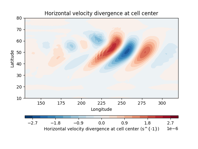
Draw a filled contour plot over a longitude-latitude subset. The helper uses the MPAS cell coordinates and supports windows that cross the dateline.

plot_cell_contourf(
    data,
    data.divergence,
    cmap = "RdBu_r",
    vmax = 3e-6,
    vmin = -3e-6,
    levels = 21,

    lon_min=130,
    lon_max=320,
    lat_min=10,
    lat_max=80,

    cbar_kwargs = {'location': 'bottom', 'aspect': 60}
)

<matplotlib.tri._tricontour.TriContourSet object at 0x73548a7f9f40>

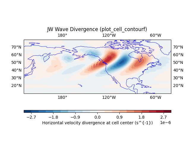
Pass an existing Cartopy axes when the contour should be combined with coastlines, gridlines, and other map decorations.

fig, ax = plt.subplots(subplot_kw= {"projection": ccrs.PlateCarree(-120)})

plot_cell_contourf(
    data,
    data.divergence,
    transform = ccrs.PlateCarree(),
    cmap = "RdBu_r",
    vmax = 3e-6,
    vmin = -3e-6,
    levels = 21,
    ax = ax,

    lon_min=130,
    lon_max=320,
    lat_min=10,
    lat_max=80,

    cbar_kwargs = {'location': 'bottom', 'aspect': 60}
)

ax.set_title("JW Wave Divergence (plot_cell_contourf)")
ax.coastlines(resolution="110m", linewidth=0.6, color = "b")
ax.gridlines(draw_labels=True, alpha = 0)

<cartopy.mpl.gridliner.Gridliner object at 0x73548b098d40>

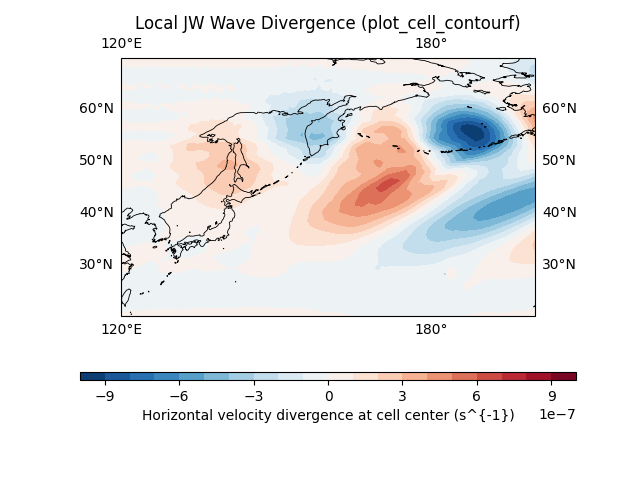
A smaller longitude-latitude window can be used to inspect regional structures without pre-slicing the MPAS mesh manually.

fig, ax = plt.subplots(subplot_kw= {"projection": ccrs.PlateCarree(160)})

plot_cell_contourf(
    data,
    data.divergence,
    transform = ccrs.PlateCarree(),
    cmap = "RdBu_r",
    levels = np.linspace(-1e-6, 1e-6, 21),
    ax = ax,

    lon_min=120,
    lon_max=200,
    lat_min=20,
    lat_max=70,

    cbar_kwargs = {'location': 'bottom', 'aspect': 60}
)

ax.set_title("Local JW Wave Divergence (plot_cell_contourf)")
ax.coastlines(resolution="50m", linewidth=0.6, color = "k")
ax.gridlines(draw_labels=True, alpha = 0)

<cartopy.mpl.gridliner.Gridliner object at 0x73548a8ab260>

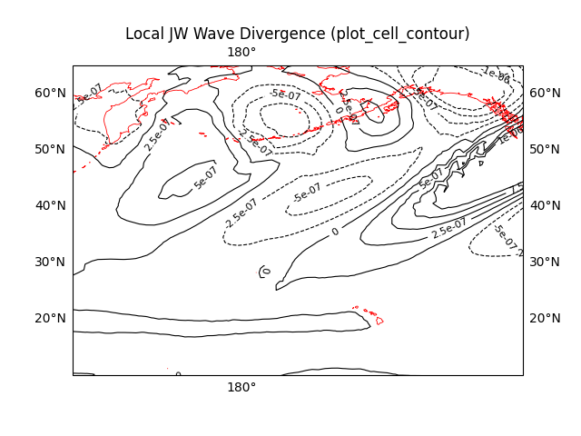
Use plot_cell_contour when contour lines and labels are preferred over a filled field.

fig, ax = plt.subplots(subplot_kw= {"projection": ccrs.PlateCarree(120)})

cs = plot_cell_contour(
    data,
    data.divergence,
    levels=np.linspace(-1e-6, 1e-6, 9),
    colors="black",
    ax=ax,
    lon_min=150,
    lon_max=230,
    lat_min=10,
    lat_max=65,
    transform=ccrs.PlateCarree(),
)
ax.clabel(cs, inline=True, fontsize=8, fmt="%g")

ax.set_title("Local JW Wave Divergence (plot_cell_contour)")
ax.coastlines(resolution="50m", linewidth=0.6, color = "r")
ax.gridlines(draw_labels=True, alpha = 0)

<cartopy.mpl.gridliner.Gridliner object at 0x73548a19f9b0>