MPAS/Voronoi grid

This example shows how to draw the edges of an MPAS Voronoi mesh with easyclimate.plot.mpas.plot_voronoi_grid.

The same mesh can be displayed on a plain Matplotlib axes or on Cartopy map projections. Longitude wrapping and dateline-crossing mesh edges are handled by the plotting helper.

import xarray as xr
import numpy as np
import cartopy.crs as ccrs
import matplotlib.pyplot as plt
import easyclimate as ecl

from easyclimate.plot.mpas import plot_voronoi_grid

Open a sample MPAS mesh dataset. The grid file contains MPAS connectivity variables such as verticesOnEdge as well as vertex coordinates.

data = ecl.open_tutorial_dataset("x1_2562_grid")
data

x1_2562_grid.nc ━━━━━━━━━━━━━━━━━━━━━━ 100.0% • 1.6/1.6 MB • 25.8 MB/s • 0:00:00

<xarray.Dataset> Size: 4MB
Dimensions:            (nCells: 2562, nVertices: 5120, nEdges: 7680,
                        maxEdges: 10, vertexDegree: 3, TWO: 2, maxEdges2: 20)
Dimensions without coordinates: nCells, nVertices, nEdges, maxEdges,
                                vertexDegree, TWO, maxEdges2
Data variables: (12/36)
    indexToCellID      (nCells) int32 10kB ...
    latCell            (nCells) float64 20kB ...
    lonCell            (nCells) float64 20kB ...
    xCell              (nCells) float64 20kB ...
    yCell              (nCells) float64 20kB ...
    zCell              (nCells) float64 20kB ...
    ...                 ...
    kiteAreasOnVertex  (nVertices, vertexDegree) float64 123kB ...
    dvEdge             (nEdges) float64 61kB ...
    dcEdge             (nEdges) float64 61kB ...
    angleEdge          (nEdges) float64 61kB ...
    weightsOnEdge      (nEdges, maxEdges2) float64 1MB ...
    meshDensity        (nCells) float64 20kB ...
Attributes:
    CDI:            Climate Data Interface version 2.4.4 (https://mpimet.mpg....
    Conventions:    CF-1.6
    mesh_spec:      1.1
    on_a_sphere:    YES
    sphere_radius:  1.0
    is_periodic:    NO
    x_period:       0.0
    y_period:       0.0
    file_id:        5d483ba2
    history:        Sat May 30 20:04:37 2026: cdo -f nc4 -z zip5 copy x1.2562...
    CDO:            Climate Data Operators version 2.4.4 (https://mpimet.mpg....

xarray.Dataset

• Dimensions:
  • nCells: 2562
  • nVertices: 5120
  • nEdges: 7680
  • maxEdges: 10
  • vertexDegree: 3
  • TWO: 2
  • maxEdges2: 20
• Data variables: (36)
  • indexToCellID
    (nCells)
    int32
    ...

    long_name :

    Mapping from local array index to global cell ID

    units :

    -

    [2562 values with dtype=int32]

  • latCell
    (nCells)
    float64
    ...

    long_name :

    Latitude of cells

    units :

    rad

    [2562 values with dtype=float64]

  • lonCell
    (nCells)
    float64
    ...

    long_name :

    Longitude of cells

    units :

    rad

    [2562 values with dtype=float64]

  • xCell
    (nCells)
    float64
    ...

    long_name :

    Cartesian x-coordinate of cells

    units :

    m

    [2562 values with dtype=float64]

  • yCell
    (nCells)
    float64
    ...

    long_name :

    Cartesian y-coordinate of cells

    units :

    m

    [2562 values with dtype=float64]

  • zCell
    (nCells)
    float64
    ...

    long_name :

    Cartesian z-coordinate of cells

    units :

    m

    [2562 values with dtype=float64]

  • indexToVertexID
    (nVertices)
    int32
    ...

    long_name :

    Mapping from local array index to global vertex ID

    units :

    -

    [5120 values with dtype=int32]

  • latVertex
    (nVertices)
    float64
    ...

    long_name :

    Latitude of vertices

    units :

    rad

    [5120 values with dtype=float64]

  • lonVertex
    (nVertices)
    float64
    ...

    long_name :

    Longitude of vertices

    units :

    rad

    [5120 values with dtype=float64]

  • xVertex
    (nVertices)
    float64
    ...

    long_name :

    Cartesian x-coordinate of vertices

    units :

    m

    [5120 values with dtype=float64]

  • yVertex
    (nVertices)
    float64
    ...

    long_name :

    Cartesian y-coordinate of vertices

    units :

    m

    [5120 values with dtype=float64]

  • zVertex
    (nVertices)
    float64
    ...

    long_name :

    Cartesian z-coordinate of vertices

    units :

    m

    [5120 values with dtype=float64]

  • indexToEdgeID
    (nEdges)
    int32
    ...

    long_name :

    Mapping from local array index to global edge ID

    units :

    -

    [7680 values with dtype=int32]

  • latEdge
    (nEdges)
    float64
    ...

    long_name :

    Latitude of edges

    units :

    rad

    [7680 values with dtype=float64]

  • lonEdge
    (nEdges)
    float64
    ...

    long_name :

    Longitude of edges

    units :

    rad

    [7680 values with dtype=float64]

  • xEdge
    (nEdges)
    float64
    ...

    long_name :

    Cartesian x-coordinate of edges

    units :

    m

    [7680 values with dtype=float64]

  • yEdge
    (nEdges)
    float64
    ...

    long_name :

    Cartesian y-coordinate of edges

    units :

    m

    [7680 values with dtype=float64]

  • zEdge
    (nEdges)
    float64
    ...

    long_name :

    Cartesian z-coordinate of edges

    units :

    m

    [7680 values with dtype=float64]

  • nEdgesOnCell
    (nCells)
    int32
    ...

    long_name :

    Number of edges forming the boundary of a cell

    units :

    -

    [2562 values with dtype=int32]

  • cellsOnCell
    (nCells, maxEdges)
    int32
    ...

    long_name :

    IDs of cells neighboring a cell

    units :

    -

    [25620 values with dtype=int32]

  • verticesOnCell
    (nCells, maxEdges)
    int32
    ...

    long_name :

    IDs of vertices (corner points) of a cell

    units :

    -

    [25620 values with dtype=int32]

  • edgesOnCell
    (nCells, maxEdges)
    int32
    ...

    long_name :

    IDs of edges forming the boundary of a cell

    units :

    -

    [25620 values with dtype=int32]

  • cellsOnVertex
    (nVertices, vertexDegree)
    int32
    ...

    long_name :

    IDs of the cells that meet at a vertex

    units :

    -

    [15360 values with dtype=int32]

  • edgesOnVertex
    (nVertices, vertexDegree)
    int32
    ...

    long_name :

    IDs of the edges that meet at a vertex

    units :

    -

    [15360 values with dtype=int32]

  • cellsOnEdge
    (nEdges, TWO)
    int32
    ...

    long_name :

    IDs of cells divided by an edge

    units :

    -

    [15360 values with dtype=int32]

  • verticesOnEdge
    (nEdges, TWO)
    int32
    ...

    long_name :

    IDs of the two vertex endpoints of an edge

    units :

    -

    [15360 values with dtype=int32]

  • nEdgesOnEdge
    (nEdges)
    int32
    ...

    long_name :

    Number of edges involved in reconstruction of tangential velocity for an edge

    units :

    -

    [7680 values with dtype=int32]

  • edgesOnEdge
    (nEdges, maxEdges2)
    int32
    ...

    long_name :

    IDs of edges involved in reconstruction of tangential velocity for an edge

    units :

    -

    [153600 values with dtype=int32]

  • areaCell
    (nCells)
    float64
    ...

    long_name :

    Spherical area of a Voronoi cell

    units :

    m^2

    [2562 values with dtype=float64]

  • areaTriangle
    (nVertices)
    float64
    ...

    long_name :

    Spherical area of a Delaunay triangle

    units :

    m^2

    [5120 values with dtype=float64]

  • kiteAreasOnVertex
    (nVertices, vertexDegree)
    float64
    ...

    long_name :

    Intersection areas between primal (Voronoi) and dual (triangular) mesh cells

    units :

    m^2

    [15360 values with dtype=float64]

  • dvEdge
    (nEdges)
    float64
    ...

    long_name :

    Spherical distance between vertex endpoints of an edge

    units :

    -

    [7680 values with dtype=float64]

  • dcEdge
    (nEdges)
    float64
    ...

    long_name :

    Spherical distance between cells separated by an edge

    units :

    m

    [7680 values with dtype=float64]

  • angleEdge
    (nEdges)
    float64
    ...

    long_name :

    Angle between local north and the positive tangential direction of an edge

    units :

    rad

    [7680 values with dtype=float64]

  • weightsOnEdge
    (nEdges, maxEdges2)
    float64
    ...

    long_name :

    Weights used in reconstruction of tangential velocity for an edge

    units :

    -

    [153600 values with dtype=float64]

  • meshDensity
    (nCells)
    float64
    ...

    long_name :

    Mesh density function (used when generating the mesh) evaluated at a cell

    units :

    unitless

    [2562 values with dtype=float64]

• Attributes: (11)

  CDI :

  Climate Data Interface version 2.4.4 (https://mpimet.mpg.de/cdi)

  Conventions :

  CF-1.6

  mesh_spec :

  1.1

  on_a_sphere :

  YES

  sphere_radius :

  1.0

  is_periodic :

  NO

  x_period :

  0.0

  y_period :

  0.0

  file_id :

  5d483ba2

  history :

  Sat May 30 20:04:37 2026: cdo -f nc4 -z zip5 copy x1.2562.grid.nc ../x1.2562.grid.nc

  CDO :

  Climate Data Operators version 2.4.4 (https://mpimet.mpg.de/cdo)

Draw the mesh directly on the current axes.

plot_voronoi_grid(data)

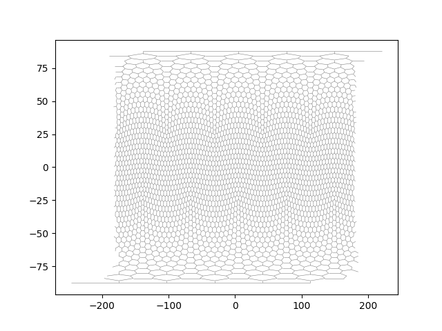
<matplotlib.collections.LineCollection object at 0x74c41a2b4830>

Plot the global mesh on a PlateCarree map. When the target axes is a Cartopy GeoAxes, the helper automatically supplies a PlateCarree transform unless a different transform is passed explicitly.

fig = plt.figure(figsize=(12, 6))
ax = plt.axes(projection=ccrs.PlateCarree(180))
ax.coastlines(resolution="110m", linewidth=0.6)

plot_voronoi_grid(data, ax = ax, transform=ccrs.PlateCarree());
ax.set_global()
ax.gridlines(draw_labels=True, alpha = 0)

ax.set_title("Global MPAS mesh 1")

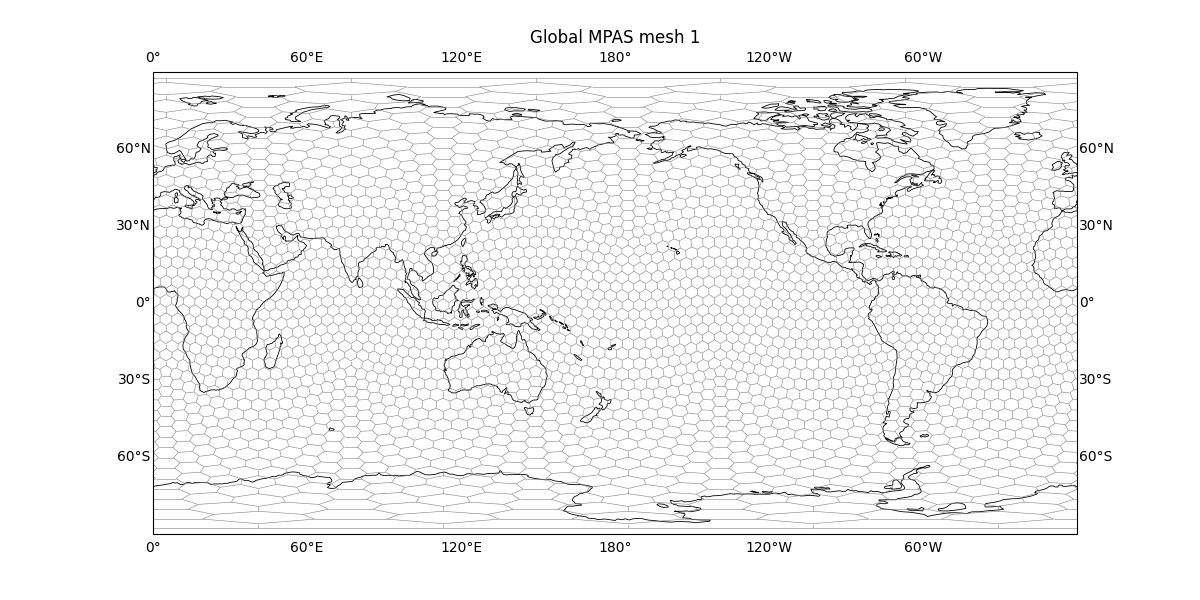
Text(0.5, 1.0453342943342954, 'Global MPAS mesh 1')

The same MPAS mesh can be displayed with another global projection.

fig = plt.figure(figsize=(12, 6))
ax = plt.axes(projection=ccrs.Robinson(0))
ax.coastlines(resolution="110m", linewidth=0.6)

plot_voronoi_grid(data, ax = ax, transform=ccrs.PlateCarree());
ax.set_global()
ax.gridlines(draw_labels=True, alpha = 0)

ax.set_title("Global MPAS mesh 2")

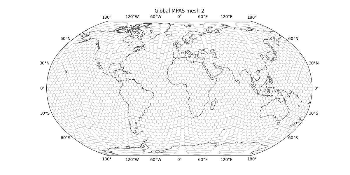
Text(0.5, 1.0453342943342951, 'Global MPAS mesh 2')

Orthographic projection is useful for inspecting a regional portion of the global unstructured grid.

fig = plt.figure(figsize=(12, 6))
ax = plt.axes(projection=ccrs.Orthographic(central_longitude=110.0, central_latitude=70.0))
ax.coastlines(resolution="110m", linewidth=0.6)

plot_voronoi_grid(data, ax = ax, transform=ccrs.PlateCarree())
ax.set_global()
ax.gridlines(draw_labels=True, alpha = 0)

ax.set_global()
ax.set_title("Global MPAS mesh 3")

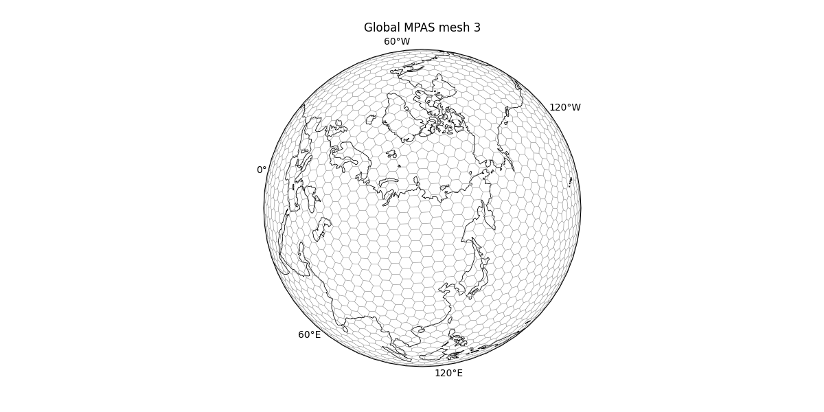
Text(0.5, 1.0381854681723834, 'Global MPAS mesh 3')