MPAS Cell-centered streamplots

This example draws streamlines from MPAS cell-centered vector winds with easyclimate.plot.mpas.plot_cell_streamplot.

The MPAS vectors are interpolated to a regular grid inside the requested longitude-latitude window before calling Matplotlib’s streamplot machinery.

import xarray as xr
import numpy as np
import cartopy.crs as ccrs
import matplotlib.pyplot as plt
import easyclimate as ecl

from easyclimate.plot.mpas import plot_cell_streamplot

Open MPAS output and select a single horizontal wind field.

data = ecl.open_tutorial_dataset("mpas_JWwave_T10_nVertLevels10")
U = data.uReconstructZonal
V = data.uReconstructMeridional

mpas_JWwave_T10_nVertLevels10.nc ━━━━━━━━ 100.0% • 2.3/2.3  • 39.2     • 0:00:00
                                                   MB         MB/s

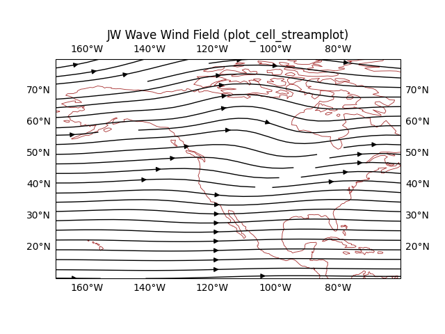
Draw streamlines over a North Pacific domain. interpolation_padding_cells adds extra source cells around the visible domain for smoother interpolation near the edges.

fig, ax = plt.subplots(subplot_kw= {"projection": ccrs.PlateCarree(-120)})

cq = plot_cell_streamplot(
    data,
    U,
    V,

    lon_min=190,
    lon_max=-60,
    lat_min=10,
    lat_max=80,

    nx=40,
    ny=20,
    density = 0.8,
    interpolation_padding_cells=10
)

ax.set_title("JW Wave Wind Field (plot_cell_streamplot)")
ax.coastlines(resolution="110m", linewidth=0.6, color = "brown")
ax.gridlines(draw_labels=True, alpha = 0)

<cartopy.mpl.gridliner.Gridliner object at 0x79225306b4d0>

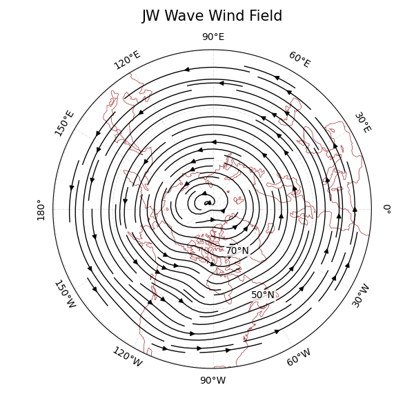
Polar streamplots can be combined with the EasyClimate polar basemap helper.

fig, ax = plt.subplots(
    figsize = (6, 6),
    subplot_kw={"projection": ccrs.NorthPolarStereo(central_longitude=-90)}
)

ax.coastlines(color="brown", linewidths=0.5)

cq = plot_cell_streamplot(
    data,
    U,
    V,

    lon_min=0,
    lon_max=359,
    lat_min=30,
    lat_max=90,

    nx=20,
    ny=18,

    title="",
    regrid_shape = 26,
)

gl, meta = ecl.plot.draw_polar_basemap(
    ax = ax,
    lon_step=30,
    lat_step=20,
    lat_range=[30, 90],
    draw_labels=True,
    gridlines_kwargs={"color": "grey", "alpha": 0.2, "linestyle": "--"},
    lat_label_lon=-60
)

ecl.plot.set_polar_title("JW Wave Wind Field", meta, size = 15)

Text(0.5, 1.0831890201695809, 'JW Wave Wind Field')