easyclimate.filter
Submodules
- easyclimate.filter.barnes_filter
- easyclimate.filter.butter_filter
- easyclimate.filter.emd
- easyclimate.filter.gaussian_filter
- easyclimate.filter.kf_filter
- easyclimate.filter.lanczos_filter
- easyclimate.filter.mask
- easyclimate.filter.redfit
- easyclimate.filter.smooth
- easyclimate.filter.spatial_pcf
- easyclimate.filter.spectrum
- easyclimate.filter.wavelet
Functions
|
Selecting different parameters g and c |
|
Select two different filtering schemes 1 and 2, and perform the filtering separately. |
|
Butterworth bandpass filter. |
|
Butterworth lowpass filter. |
|
Butterworth highpass filter. |
|
Lanczos bandpass filter |
|
Lanczos lowpass filter |
|
Lanczos highpass filter |
Filter with normal distribution of weights. |
|
Filter with a rectangular window smoother. |
|
Filter with an 5-point or 9-point smoother. |
|
|
Filter with the forward smooth. |
|
Filter with the reverse smooth. |
Filter with a circular window smoother. |
|
Filter with an arbitrary window smoother. |
|
|
Wavelet transform parameters calculation. |
|
Draw global wavelet spectrum |
|
Draw wavelet transform |
|
Estimating red-noise spectra directly from unevenly spaced paleoclimatic time series. |
|
Estimating red-noise spectra directly from unevenly spaced paleoclimatic time series. |
|
Extract equatorial waves by filtering in the Wheeler-Kiladis wavenumber-frequency domain. |
|
Extract low-frequency waves by filtering in the Wheeler-Kiladis wavenumber-frequency domain. The maximum period is beyond 120 days. |
|
Extract Madden-Julian Oscillation (MJO) waves by filtering in the Wheeler-Kiladis wavenumber-frequency domain |
|
Extract equatorial Rossby (ER) waves by filtering in the Wheeler-Kiladis wavenumber-frequency domain. |
|
Extract Kelvin waves by filtering in the Wheeler-Kiladis wavenumber-frequency domain. |
|
Extract mixed Rossby-gravity (MRG)-tropical depression (TD) type waves by filtering in the Wheeler-Kiladis wavenumber-frequency domain |
|
Extract mixed Rossby-gravity waves (MRG) by filtering in the Wheeler-Kiladis wavenumber-frequency domain. |
|
Extract tropical depression (TD) by filtering in the Wheeler-Kiladis wavenumber-frequency domain. |
|
Perform space-time spectral analysis to extract equatorial wave components. |
|
Empirical Mode Decomposition |
|
Ensemble Empirical Mode Decomposition (EEMD) |
|
Apply a Gaussian filter to data along a specified dimension. |
|
Calculate the time spectrum of a multi-dimensional |
|
Calculate mean Fourier amplitude between specified period bounds. |
|
Apply Fourier harmonic analysis to filter an dataset along a time dimension. |
|
Generate a mask for a custom geographical rectangular box with optional rotation. |
Package Contents
- easyclimate.filter.calc_barnes_lowpass(data: xarray.DataArray, g: float = 0.3, c: int = 150000, lon_dim='lon', lat_dim='lat', radius_degree=8, print_progress=True) xarray.DataArray
Selecting different parameters g and c will result in different filtering characteristics.
Warning
NOT support
datacontainsnp.nan.Parameters
- data
xarray.DataArray. The spatio-temporal data to be calculated.
- g
float, generally between (0, 1], default 0.3. Constant parameter.
- c
int, default 150000. Constant parameter. When c takes a larger value, the filter function converges at a larger wavelength, and the response function slowly approaches the maximum value, which means that high-frequency fluctuations have been filtered out.
- lon_dim:
str, default: lon. Longitude coordinate dimension name. By default extracting is applied over the lon dimension.
- lat_dim:
str, default: lat. Latitude coordinate dimension name. By default extracting is applied over the lat dimension.
- radius_degree
intortuple(degree), default 8. The radius of each point when caculating the distance of each other.
It is recommended to set this with your schemes. For the constant
c, this parameter is recommended to be:for the
cis[500, 1000, 2000, 5000, 10000, 20000, 50000, 100000, 200000]radius_degreeis recommended for[1, 1.5, 2, 3, 4, 5, 7, 8, 12]- print_progress
bool Whether to print the progress bar when executing computation.
Returns
- data_vars
xarray.DataArray Data field after filtering out high-frequency fluctuations
See also
Maddox, R. A. (1980). An Objective Technique for Separating Macroscale and Mesoscale Features in Meteorological Data. Monthly Weather Review, 108(8), 1108-1121. https://journals.ametsoc.org/view/journals/mwre/108/8/1520-0493_1980_108_1108_aotfsm_2_0_co_2.xml
- data

- easyclimate.filter.calc_barnes_bandpass(data: xarray.DataArray, g1: float = 0.3, g2: float = 0.3, c1: int = 30000, c2: int = 150000, r=1.2, lon_dim='lon', lat_dim='lat', radius_degree=8, print_progress=True) xarray.DataArray
Select two different filtering schemes 1 and 2, and perform the filtering separately. And then perform the difference, that means scheme1 - scheme2. The mesoscale fluctuations are thus preserved.
Warning
NOT support
datacontainsnp.nan.Parameters
- data
xarray.DataArray. The spatio-temporal data to be calculated.
- g1
float, generally between (0, 1], default 0.3. Constant parameter of scheme1.
- g2
float, generally between (0, 1], default 0.3. Constant parameter of scheme2.
- c1
int, default 30000. Constant parameterof scheme1.
- c2
int, default 150000. Constant parameterof scheme2.
- r
float, default 1.2. The inverse of the maximum response differenc. It is prevented from being unduly large and very small difference fields are not greatly amplified.
- lon_dim:
str, default: lon. Longitude coordinate dimension name. By default extracting is applied over the lon dimension.
- lat_dim:
str, default: lat. Latitude coordinate dimension name. By default extracting is applied over the lat dimension.
- radius_degree
intortuple(degree), default 8. The radius of each point when caculating the distance of each other.
It is recommended to set this with your schemes. For the constant
c, this parameter is recommended to be:for the
cis[500, 1000, 2000, 5000, 10000, 20000, 50000, 100000, 200000],radius_degreeis recommended for[1, 1.5, 2, 3, 4, 5, 7, 8, 12]- print_progress
bool Whether to print the progress bar when executing computation.
Returns
- data_vars
xarray.DataArray Mesoscale wave field filtered out from raw data
See also
Maddox, R. A. (1980). An Objective Technique for Separating Macroscale and Mesoscale Features in Meteorological Data. Monthly Weather Review, 108(8), 1108-1121. https://journals.ametsoc.org/view/journals/mwre/108/8/1520-0493_1980_108_1108_aotfsm_2_0_co_2.xml
- data
- easyclimate.filter.calc_butter_bandpass(data: xarray.DataArray | xarray.Dataset, sampling_frequency: int, period: list[int], N: int = 3, dim: str = 'time') xarray.DataArray
Butterworth bandpass filter.
Parameters
- data:
xarray.DataArrayorxarray.Dataset. The array of data to be filtered.
- sampling_frequency:
int. Data sampling frequency. If it is daily data with only one time level record per day, then the parameter value is 1; If a day contains four time level records, the parameter value is 4.
- period:
list[int]. The time period interval of the bandpass filter to be acquired. If we are obtaining a 3-10 day bandpass filter, the value of this parameter is [3, 10]. Note that the units of this parameter should be consistent with sampling_frequency.
- N:
int. The order of the filter. Default is 3.
- dim:
str.. Dimension(s) over which to apply bandpass filter. By default gradient is applied over the time dimension.
See also
- data:
- easyclimate.filter.calc_butter_lowpass(data: xarray.DataArray | xarray.Dataset, sampling_frequency: int, period: float, N: int = 3, dim: str = 'time') xarray.DataArray
Butterworth lowpass filter.
Parameters
- data:
xarray.DataArrayorxarray.Dataset. The array of data to be filtered.
- sampling_frequency:
int. Data sampling frequency. If it is daily data with only one time level record per day, then the parameter value is 1; If a day contains four time level records, the parameter value is 4.
- period:
float. The low-pass filtering time period, above which the signal (low frequency signal) will pass. If you are getting a 10-day low-pass filter, the value of this parameter is 10. Note that the units of this parameter should be consistent with sampling_frequency.
- N:
int. The order of the filter. Default is 3.
- dim:
str.. Dimension(s) over which to apply lowpass filter. By default gradient is applied over the time dimension.
See also
- data:
- easyclimate.filter.calc_butter_highpass(data: xarray.DataArray | xarray.Dataset, sampling_frequency: int, period: float, N: int = 3, dim: str = 'time') xarray.DataArray
Butterworth highpass filter.
Parameters
- data:
xarray.DataArrayorxarray.Dataset. The array of data to be filtered.
- sampling_frequency:
int. Data sampling frequency. If it is daily data with only one time level record per day, then the parameter value is 1; If a day contains four time level records, the parameter value is 4.
- period:
float. The high-pass filtering time period below which the signal (high-frequency signal) will pass. If you are obtaining a 10-day high-pass filter, the value of this parameter is 10. Note that the units of this parameter should be consistent with sampling_frequency.
- N:
int. The order of the filter. Default is 3.
- dim:
str.. Dimension(s) over which to apply highpass filter. By default gradient is applied over the time dimension.
See also
- data:
- easyclimate.filter.calc_lanczos_bandpass(data: xarray.DataArray | xarray.Dataset, window_length: int, period: list[int], dim: str = 'time', method: Literal['rolling', 'convolve'] = 'rolling', drop_edge: bool = True) xarray.DataArray
Lanczos bandpass filter
- data:
xarray.DataArrayorxarray.Dataset. The array of data to be filtered.
- window_length:
int. Slide the size of the window.
- period:
list[int]. The time period interval of the bandpass filter to be acquired. If we are obtaining a 3-10 day bandpass filter, the value of this parameter is [3, 10].
- dim:
str. Dimension(s) over which to apply bandpass filter. By default gradient is applied over the time dimension.
- method:
str, default: rolling. Filter method. Optional values are rolling, convolve.
- data:
- easyclimate.filter.calc_lanczos_lowpass(data: xarray.DataArray | xarray.Dataset, window_length: int, period: int, dim: str = 'time', method: Literal['rolling', 'convolve'] = 'rolling', drop_edge: bool = True) xarray.DataArray
Lanczos lowpass filter
- data:
xarray.DataArrayorxarray.Dataset. The array of data to be filtered.
- window_length:
int. Slide the size of the window.
- period:
float. The low-pass filtering time period, above which the signal (low frequency signal) will pass. If you are getting a 10-day low-pass filter, the value of this parameter is 10.
- dim:
str. Dimension(s) over which to apply lowpass filter. By default gradient is applied over the time dimension.
- method:
str, default: rolling. Filter method. Optional values are rolling, convolve.
- data:
- easyclimate.filter.calc_lanczos_highpass(data: xarray.DataArray | xarray.Dataset, window_length: int, period: int, dim: str = 'time', method: Literal['rolling', 'convolve'] = 'rolling', drop_edge: bool = True) xarray.DataArray
Lanczos highpass filter
- data:
xarray.DataArrayorxarray.Dataset. The array of data to be filtered.
- window_length:
int. Slide the size of the window.
- period:
int. The high-pass filtering time period below which the signal (high-frequency signal) will pass. If you are obtaining a 10-day high-pass filter, the value of this parameter is 10.
- dim:
str. Dimension(s) over which to apply highpass filter. By default gradient is applied over the time dimension.
- method:
str, default: rolling. Filter method. Optional values are rolling, convolve.
- data:
- easyclimate.filter.calc_spatial_smooth_gaussian(data: xarray.DataArray | xarray.Dataset, n: int = 3, lon_dim: str = 'lon', lat_dim: str = 'lat') xarray.DataArray | xarray.Dataset
Filter with normal distribution of weights.
Parameters
- data:
xarray.DataArrayorxarray.Dataset. Some n-dimensional latitude-longitude dataset.
- n:
int. Degree of filtering.
Returns
The filtered latitude-longitude dataset (
xarray.DataArrayorxarray.Dataset).- data:
- easyclimate.filter.calc_spatial_smooth_rectangular(data: xarray.DataArray | xarray.Dataset, rectangle_shapes: int | Sequence[int] = 3, times: int = 1, lon_dim: str = 'lon', lat_dim: str = 'lat') xarray.DataArray | xarray.Dataset
Filter with a rectangular window smoother.
Parameters
- data:
xarray.DataArrayorxarray.Dataset. Some n-dimensional latitude-longitude dataset.
- rectangle_shapes:
intorSequence[int], default 3. Shape of rectangle along the trailing dimension(s) of the data.
- times:
intor , default 1. The number of times to apply the filter to the data.
- lon_dim:
str, default: lon. Longitude coordinate dimension name. By default extracting is applied over the lon dimension.
- lat_dim:
str, default: lat. Latitude coordinate dimension name. By default extracting is applied over the lat dimension.
Returns
The filtered latitude-longitude dataset (
xarray.DataArrayorxarray.Dataset).- data:
- easyclimate.filter.calc_spatial_smooth_5or9_point(data: xarray.DataArray | xarray.Dataset, n: {5, 9} = 5, times: int = 1, lon_dim: str = 'lon', lat_dim: str = 'lat') xarray.DataArray | xarray.Dataset
Filter with an 5-point or 9-point smoother.
Parameters
- data:
xarray.DataArrayorxarray.Dataset. Some n-dimensional latitude-longitude dataset.
- n: {5, 9}, default 5.
The number of points to use in smoothing, only valid inputs are 5 and 9.
- times:
intor , default 1. The number of times to apply the filter to the data.
- lon_dim:
str, default: lon. Longitude coordinate dimension name. By default extracting is applied over the lon dimension.
- lat_dim:
str, default: lat. Latitude coordinate dimension name. By default extracting is applied over the lat dimension.
Returns
The filtered latitude-longitude dataset (
xarray.DataArrayorxarray.Dataset).- data:
- easyclimate.filter.calc_forward_smooth(data: xarray.DataArray | xarray.Dataset, n: int = 5, S: float = 0.5, times: int = 1, normalize_weights=False, lon_dim: str = 'lon', lat_dim: str = 'lat') xarray.DataArray | xarray.Dataset
Filter with the forward smooth.
Parameters
- data:
xarray.DataArrayorxarray.Dataset. Some n-dimensional latitude-longitude dataset.
- n: {5, 9}, default 5.
The number of points to use in smoothing, only valid inputs are 5 and 9.
- S:
float, default 0.5. The smoothing factor.
- times:
int, default 1. The number of times to apply the filter to the data.
- normalize_weights:
bool, default False. If True, divide the values in window by the sum of all values in the window to obtain the normalized smoothing weights. If False, use supplied values directly as the weights.
- lon_dim:
str, default: lon. Longitude coordinate dimension name. By default extracting is applied over the lon dimension.
- lat_dim:
str, default: lat. Latitude coordinate dimension name. By default extracting is applied over the lat dimension.
Returns
The filtered latitude-longitude dataset (
xarray.DataArrayorxarray.Dataset).Note
For any discrete variable, its value on the \(x\)-axis can be described as \(F_i = F(x_i)\), where \(x_i = i \Delta x, i = 0, \pm 1, \pm 2\).
Define a one-dimensional smoothing operator
\[\overset{\sim}{F}_{i}^x = (1-S)F_i + \frac{S}{2} (F_{i+1} + F_{i-1})\]Here, \(S\) is the spatial smoothing coefficient. Since the above formula only involves the values of three grid data points (\(F_i, F_{i+1}, F_{i-1}\)), it is also referred to as a three-point smoothing.
Correspondingly, for a two-dimensional variable \(F_{i,j}\), smoothing is performed in the \(x\) direction as follows
\[\overset{\sim}{F}_{i,j}^x = F_{i,j} + \frac{S}{2} (F_{i+1,j} + F_{i-1,j}-2F_{i,j})\]And, smoothing is done in the \(y\) direction separately
\[\overset{\sim}{F}_{i,j}^y = F_{i,j} + \frac{S}{2} (F_{i,j+1} + F_{i,j-1}-2F_{i,j})\]Taking the average of both results:
\[\overset{\sim}{F}_{i,j}^{x,y} = \frac{\overset{\sim}{F}_{i,j}^x + \overset{\sim}{F}_{i,j}^y}{2} = F_{i,j} + \frac{S}{4}(F_{i+1,j}+F_{i,j+1}+F_{i-1,j}+F_{i,j-1}-4F_{i,j})\]At this point, the following “window” matrix \(\mathbf{W}\) can be obtained
\[\begin{split}\mathbf{W} = \left( \begin{array}{ccc} F_{i-1,j+1} & F_{i,j+1} & F_{i+1,j+1} \\ F_{i-1,j} & F_{i,j} & F_{i+1,j} \\ F_{i-1,j-1} & F_{i,j-1} & F_{i+1,j-1} \end{array} \right) = \left( \begin{array}{ccc} 0 & \frac{S}{4} & 0 \\ \frac{S}{4} & (1-S) & \frac{S}{4} \\ 0 & \frac{S}{4} & 0 \end{array} \right)\end{split}\]When \(S=0.5\), we have
\[\begin{split}\mathbf{W} = \left( \begin{array}{ccc} 0 & 0.125 & 0 \\ 0.125 & 0.5 & 0.125 \\ 0 & 0.125 & 0 \end{array} \right)\end{split}\]This is the “window” matrix used by the function when \(n=5\).
For the variable \(F_{i,j}\), applying a three-point smoothing in the \(x\)-axis direction followed by a three-point smoothing in the \(y\)-axis direction results in the following nine-point smoothing scheme
\[\overset{\sim}{F}_{i,j}^{x,y} = {F}_{i,j} + \frac{S}{2}(1-S)(F_{i+1,j}+F_{i,j+1}+F_{i-1,j}+F_{i,j-1}-4F_{i,j})+\frac{S^2}{4}(F_{i+1,j+1}+F_{i-1,j+1}+F_{i-1,j-1}+F_{i+1,j-1}-4F_{i,j})\]At this point, the corresponding “window” matrix \(\mathbf{W}\) is given by
\[\begin{split}\mathbf{W} = \left( \begin{array}{ccc} F_{i-1,j+1} & F_{i,j+1} & F_{i+1,j+1} \\ F_{i-1,j} & F_{i,j} & F_{i+1,j} \\ F_{i-1,j-1} & F_{i,j-1} & F_{i+1,j-1} \end{array} \right) = \left( \begin{array}{ccc} \frac{S^2}{4} & \frac{S}{2}(1-S) & \frac{S^2}{4} \\ \frac{S}{2}(1-S) & 1-2S(1-S) & \frac{S}{2}(1-S) \\ \frac{S^2}{4} & \frac{S}{2}(1-S) & \frac{S^2}{4} \end{array} \right)\end{split}\]When \(S=0.5\), we have
\[\begin{split}\mathbf{W} = \left( \begin{array}{ccc} 0.0625 & 0.125 & 0.0625 \\ 0.125 & 0.5 & 0.125 \\ 0.0625 & 0.125 & 0.0625 \end{array} \right)\end{split}\]This is the “window” matrix used by the function when \(n=9\).
See also
- data:
- easyclimate.filter.calc_reverse_smooth(data: xarray.DataArray | xarray.Dataset, n: int = 5, S: float = -0.5, times: int = 1, normalize_weights=False, lon_dim: str = 'lon', lat_dim: str = 'lat') xarray.DataArray | xarray.Dataset
Filter with the reverse smooth.
Parameters
- data:
xarray.DataArrayorxarray.Dataset. Some n-dimensional latitude-longitude dataset.
- n: {5, 9}, default 5.
The number of points to use in smoothing, only valid inputs are 5 and 9.
- S:
float, default -0.5. The smoothing factor.
- times:
int, default 1. The number of times to apply the filter to the data.
- normalize_weights:
bool, default False. If True, divide the values in window by the sum of all values in the window to obtain the normalized smoothing weights. If False, use supplied values directly as the weights.
- lon_dim:
str, default: lon. Longitude coordinate dimension name. By default extracting is applied over the lon dimension.
- lat_dim:
str, default: lat. Latitude coordinate dimension name. By default extracting is applied over the lat dimension.
Returns
The filtered latitude-longitude dataset (
xarray.DataArrayorxarray.Dataset).Note
For any discrete variable, its value on the \(x\)-axis can be described as \(F_i = F(x_i)\), where \(x_i = i \Delta x, i = 0, \pm 1, \pm 2\).
Define a one-dimensional smoothing operator
\[\overset{\sim}{F}_{i}^x = (1-S)F_i + \frac{S}{2} (F_{i+1} + F_{i-1})\]Here, \(S\) is the spatial smoothing coefficient. Since the above formula only involves the values of three grid data points (\(F_i, F_{i+1}, F_{i-1}\)), it is also referred to as a three-point smoothing.
Correspondingly, for a two-dimensional variable \(F_{i,j}\), smoothing is performed in the \(x\) direction as follows
\[\overset{\sim}{F}_{i,j}^x = F_{i,j} + \frac{S}{2} (F_{i+1,j} + F_{i-1,j}-2F_{i,j})\]And, smoothing is done in the \(y\) direction separately
\[\overset{\sim}{F}_{i,j}^y = F_{i,j} + \frac{S}{2} (F_{i,j+1} + F_{i,j-1}-2F_{i,j})\]Taking the average of both results:
\[\overset{\sim}{F}_{i,j}^{x,y} = \frac{\overset{\sim}{F}_{i,j}^x + \overset{\sim}{F}_{i,j}^y}{2} = F_{i,j} + \frac{S}{4}(F_{i+1,j}+F_{i,j+1}+F_{i-1,j}+F_{i,j-1}-4F_{i,j})\]At this point, the following “window” matrix \(\mathbf{W}\) can be obtained
\[\begin{split}\mathbf{W} = \left( \begin{array}{ccc} F_{i-1,j+1} & F_{i,j+1} & F_{i+1,j+1} \\ F_{i-1,j} & F_{i,j} & F_{i+1,j} \\ F_{i-1,j-1} & F_{i,j-1} & F_{i+1,j-1} \end{array} \right) = \left( \begin{array}{ccc} 0 & \frac{S}{4} & 0 \\ \frac{S}{4} & (1-S) & \frac{S}{4} \\ 0 & \frac{S}{4} & 0 \end{array} \right)\end{split}\]When \(S=0.5\), we have
\[\begin{split}\mathbf{W} = \left( \begin{array}{ccc} 0 & 0.125 & 0 \\ 0.125 & 0.5 & 0.125 \\ 0 & 0.125 & 0 \end{array} \right)\end{split}\]This is the “window” matrix used by the function when \(n=5\).
For the variable \(F_{i,j}\), applying a three-point smoothing in the \(x\)-axis direction followed by a three-point smoothing in the \(y\)-axis direction results in the following nine-point smoothing scheme
\[\overset{\sim}{F}_{i,j}^{x,y} = {F}_{i,j} + \frac{S}{2}(1-S)(F_{i+1,j}+F_{i,j+1}+F_{i-1,j}+F_{i,j-1}-4F_{i,j})+\frac{S^2}{4}(F_{i+1,j+1}+F_{i-1,j+1}+F_{i-1,j-1}+F_{i+1,j-1}-4F_{i,j})\]At this point, the corresponding “window” matrix \(\mathbf{W}\) is given by
\[\begin{split}\mathbf{W} = \left( \begin{array}{ccc} F_{i-1,j+1} & F_{i,j+1} & F_{i+1,j+1} \\ F_{i-1,j} & F_{i,j} & F_{i+1,j} \\ F_{i-1,j-1} & F_{i,j-1} & F_{i+1,j-1} \end{array} \right) = \left( \begin{array}{ccc} \frac{S^2}{4} & \frac{S}{2}(1-S) & \frac{S^2}{4} \\ \frac{S}{2}(1-S) & 1-2S(1-S) & \frac{S}{2}(1-S) \\ \frac{S^2}{4} & \frac{S}{2}(1-S) & \frac{S^2}{4} \end{array} \right)\end{split}\]When \(S=0.5\), we have
\[\begin{split}\mathbf{W} = \left( \begin{array}{ccc} 0.0625 & 0.125 & 0.0625 \\ 0.125 & 0.5 & 0.125 \\ 0.0625 & 0.125 & 0.0625 \end{array} \right)\end{split}\]This is the “window” matrix used by the function when \(n=9\).
See also
- data:
- easyclimate.filter.calc_spatial_smooth_circular(data: xarray.DataArray | xarray.Dataset, radius: int, times: int = 1, lon_dim: str = 'lon', lat_dim: str = 'lat') xarray.DataArray | xarray.Dataset
Filter with a circular window smoother.
Parameters
- data:
xarray.DataArrayorxarray.Dataset. Some n-dimensional latitude-longitude dataset.
- radius:
int. Radius of the circular smoothing window. The “diameter” of the circle (width of smoothing window) is \(2 \cdot \mathrm{radius} + 1\) to provide a smoothing window with odd shape.
- times:
int, default 1. The number of times to apply the filter to the data.
- lon_dim:
str, default: lon. Longitude coordinate dimension name. By default extracting is applied over the lon dimension.
- lat_dim:
str, default: lat. Latitude coordinate dimension name. By default extracting is applied over the lat dimension.
Returns
The filtered latitude-longitude dataset (
xarray.DataArrayorxarray.Dataset).- data:
- easyclimate.filter.calc_spatial_smooth_window(data: xarray.DataArray | xarray.Dataset, window: numpy.ndarray | xarray.DataArray, times: int = 1, normalize_weights: bool = False, lon_dim: str = 'lon', lat_dim: str = 'lat') xarray.DataArray | xarray.Dataset
Filter with an arbitrary window smoother.
Parameters
- data:
xarray.DataArrayorxarray.Dataset. Some n-dimensional latitude-longitude dataset.
- window
numpy.ndarrayorxarray.DataArray. Window to use in smoothing. Can have dimension less than or equal to \(N\). If dimension less than \(N\), the scalar grid will be smoothed along its trailing dimensions. Shape along each dimension must be odd.
- times:
int, default 1. The number of times to apply the filter to the data.
- normalize_weights:
bool, default False. If True, divide the values in window by the sum of all values in the window to obtain the normalized smoothing weights. If False, use supplied values directly as the weights.
- lon_dim:
str, default: lon. Longitude coordinate dimension name. By default extracting is applied over the lon dimension.
- lat_dim:
str, default: lat. Latitude coordinate dimension name. By default extracting is applied over the lat dimension.
Returns
The filtered latitude-longitude dataset (
xarray.DataArrayorxarray.Dataset).- data:
- easyclimate.filter.calc_timeseries_wavelet_transform(timeseries_data: xarray.DataArray, dt: float, time_dim: str = 'time', pad: float = 1, dj: float = 0.25, j1_n_div_dj: int = 7, s0=None, lag1: float = None, mother: str = 'morlet', mother_param=None, sigtest_wavelet: str = 'regular chi-square test', sigtest_global: str = 'time-average test', significance_level: float = 0.95) xarray.Dataset
Wavelet transform parameters calculation.
Parameters
- timeseries_data:
xarray.DataArray. Timeseries data.
- dt:
float. Amount of time between each timeseries data value, i.e. the sampling time.
- time_dim:
str. The time coordinate dimension name.
- pad:
float, default: 1. if set to 1 (default is 0), pad time series with zeroes to get N up to the next higher power of 2. This prevents wraparound from the end of the time series to the beginning, and also speeds up the FFT’s used to do the wavelet transform. This will not eliminate all edge effects (see COI below).
- dj:
float, default: 0.25. The spacing between discrete scales. A smaller dj will give better scale resolution, but be slower to plot.
- j1_n_div_dj:
int, default: 7. Do j1_n_div_dj powers-of-two with dj sub-octaves each.
\[j1 = \mathrm{j1\underline{ }n\underline{ }div\underline{ }dj} / dj\]This can adjust the size of the period.
- s0:
float, default: \(2 \times \mathrm{d}t\). The smallest scale of the wavelet.
- lag1:
float, default: None. Lag-1 autocorrelation for red noise background. The value is generated by
statsmodels.api.tsa.acf.- mother:
str, {‘morlet’, ‘paul’, ‘dog’}, default: ‘morlet’. The mother wavelet function.
Name: Morlet (\(\omega_0\) = frequency)
\(\psi_0(\eta)\): \(\pi^{-1/4} e^{i \omega_{0} \eta} e^{-\eta^2/2}\).
Name: Paul (\(m\) = order)
\(\psi_0(\eta)\): \(\frac{2^m i^m m!}{\sqrt{\pi (2m)!}} (1-i \eta)^{-(m+1)}\).
Name: DOG (\(m\) = derivative)
\(\psi_0(\eta)\): \(\frac{(-1)^{m+1}}{\sqrt{\Gamma (m+\frac{1}{2})}} \frac{d^m}{d \eta^m} (e^{-\eta^2 /2})\).
- mother_param:
float. - The mother wavelet parameter.
For ‘morlet’ this is \(k_0\) (wavenumber), default is 6.
For ‘paul’ this is \(m\) (order), default is 4.
For ‘dog’ this is \(m\) (m-th derivative), default is 2.
- sigtest_wavelet: {‘regular chi-square test’, ‘time-average test’, ‘scale-average test’}, default: ‘regular chi-square test’.
The type of significance test.
1. Regular chi-square test i.e. Eqn (18) from Torrence & Compo.
\[\frac{\left|W_n(s)\right|^2}{\sigma^2}\Longrightarrow\frac{1}{2} P_k\chi_2^2\]The “time-average” test, i.e. Eqn (23).
\[\nu=2\sqrt{1+\left(\frac{n_a\delta t}{\gamma s}\right)^2}\]In this case, DOF should be set to NA, the number of local wavelet spectra that were averaged together. For the Global Wavelet Spectrum, this would be NA=N, where N is the number of points in your time series.
The “scale-average” test, i.e. Eqns (25)-(28).
\[\overline{P}=S_{\mathrm{avg}}\sum_{j=j_1}^{j_2}\frac{P_j}{S_j}, \ \mathrm{where} \ S_{\mathrm{avg}}=\left(\sum_{j=j_1}^{j_2}\frac1{s_j}\right)^{-1}, \frac{C_\delta S_\mathrm{avg}}{\delta j\delta t\sigma^2}\overline{W}_n^2\Rightarrow\overline{P}\frac{\chi_\nu^2}\nu, \nu=\frac{2n_aS_{\mathrm{avg}}}{S_{\mathrm{mid}}}\sqrt{1+\left(\frac{n_a\delta j}{\delta j_0}\right)^2}.\]In this case, DOF should be set to a two-element vector [S1,S2], which gives the scale range that was averaged together. e.g. if one scale-averaged scales between 2 and 8, then DOF=[2,8].
- sigtest_global: {‘regular chi-square test’, ‘time-average test’, ‘scale-average test’}, default: ‘time-average test’.
See also the description of sigtest_wavelet.
- significance_level:
float, default: 0.95. Significance level to use.
Returns
Timeseries wavelet transform result (
xarray.Dataset).Reference
Torrence, C., & Compo, G. P. (1998). A Practical Guide to Wavelet Analysis. Bulletin of the American Meteorological Society, 79(1), 61-78. https://doi.org/10.1175/1520-0477(1998)079<0061:APGTWA>2.0.CO;2
Torrence, C., & Webster, P. J. (1999). Interdecadal Changes in the ENSO–Monsoon System. Journal of Climate, 12(8), 2679-2690. https://doi.org/10.1175/1520-0442(1999)012<2679:ICITEM>2.0.CO;2
Grinsted, A., Moore, J. C., and Jevrejeva, S.: Application of the cross wavelet transform and wavelet coherence to geophysical time series, Nonlin. Processes Geophys., 11, 561–566, https://doi.org/10.5194/npg-11-561-2004, 2004.
- timeseries_data:

- easyclimate.filter.draw_global_wavelet_spectrum(timeseries_wavelet_transform_result: xarray.Dataset, ax: matplotlib.axes.Axes = None, global_ws_kwargs: dict = {}, global_signif_kwargs: dict = {'ls': '--'})
Draw global wavelet spectrum
Parameters
- timeseries_wavelet_transform_result:
xarray.Dataset. Timeseries wavelet transform result.
- ax:
matplotlib.axes.Axes The axes to which the boundary will be applied.
- **global_ws_kwargs,
dict, optional: Additional keyword arguments to
xarray.DataArray.plot.linefor ploting global_ws.- **global_signif_kwargs,
dict, optional, default {‘ls’: ‘–‘}: Additional keyword arguments to
xarray.DataArray.plot.linefor ploting global_signif.
- timeseries_wavelet_transform_result:
- easyclimate.filter.draw_wavelet_transform(timeseries_wavelet_transform_result: xarray.Dataset, ax: matplotlib.axes.Axes = None, power_kwargs: dict = {'levels': [0, 0.5, 1, 2, 4, 999], 'colors': ['white', 'bisque', 'orange', 'orangered', 'darkred']}, sig_kwargs: dict = {'levels': [-99, 1], 'colors': 'k'}, coi_kwargs: dict = {'color': 'k'}, fill_between_kwargs: dict = {'facecolor': 'none', 'edgecolor': '#00000040', 'hatch': 'x'})
Draw wavelet transform
Parameters
- timeseries_wavelet_transform_result:
xarray.Dataset. Timeseries wavelet transform result.
- ax
matplotlib.axes.Axes The axes to which the boundary will be applied.
- **power_kwargs, optional,
dict, default {‘levels’: [0, 0.5, 1, 2, 4, 999], ‘colors’: [‘white’, ‘bisque’, ‘orange’, ‘orangered’, ‘darkred’]}: Additional keyword arguments to
xarray.DataArray.plot.contourffor ploting power.- **sig_kwargs, optional,
dict, default {‘levels’: [-99, 1], ‘colors’: ‘k’}: Additional keyword arguments to
xarray.DataArray.plot.contourffor ploting sig.- **coi_kwargs, optional,
dict, default {‘color’: ‘k’}: Additional keyword arguments to
xarray.DataArray.plot.contourffor ploting coi.- **fill_between_kwargs,
dict, optional, default {‘facecolor’: ‘none’, ‘edgecolor’: ‘#00000040’, ‘hatch’: ‘x’}: Additional keyword arguments to
matplotlib.pyplot.fill_between.
- timeseries_wavelet_transform_result:
- easyclimate.filter.calc_redfit(data: xarray.DataArray, timearray: numpy.array = None, nsim: int = 1000, mctest: bool = False, rhopre: float = -99.0, ofac: float = 1.0, hifac: float = 1.0, n50: int = 1, iwin: Literal['rectangular', 'welch', 'hanning', 'triangular', 'blackmanharris'] = 'rectangular')
Estimating red-noise spectra directly from unevenly spaced paleoclimatic time series.
Parameters
- data:
xarray.DataArray Input time series data
- timearray:
numpy.array Time series data array
- nsim:
int Number of Monte-Carlo simulations (1000-2000 should be o.k. in most cases)
- mctest:
bool Toggle calculation of false-alarm levels based on Monte-Carlo simulation, if set to True : perform Monte-Carlo test, if set to False : skip Monte-Carlo test (default).
- rhopre:
float Prescibed value for \(\rho\); unused if < 0 (default = -99.0)
- ofac:
float Oversampling factor for Lomb-Scargle Fourier transform (typical values: 2.0-4.0)
- hifac:
float Max. frequency to analyze is set to hifac * <fNyq> (default = 1.0)
- n50:
int Number of WOSA segments (with 50 % overlap)
- iwin: {“rectangular”, “welch”, “hanning”, “triangular”, “blackmanharris”}
Window-type identifier used to suppress sidelobes in spectral analysis: ({“rectangular”, “welch”, “hanning”, “triangular”, “blackmanharris”}, optional)
Caution
Parameters ofac, hifac, n50 and window type are identical to the SPECTRUM program (see Schulz and Stattegger, 1997 for further details). Except mctest, hifac and rhopre all parameters must be specified.
Returns
The red-noise spectra (
xarray.Dataset).See also
Schulz, M., & Mudelsee, M. (2002). REDFIT: estimating red-noise spectra directly from unevenly spaced paleoclimatic time series [Software]. Computers & Geosciences, 28(3), 421-426. https://doi.org/10.1016/S0098-3004(01)00044-9
https://www.marum.de/Prof.-Dr.-michael-schulz/Michael-Schulz-Software.html
- data:
- easyclimate.filter.calc_redfit_cross(data_x: xarray.DataArray, data_y: xarray.DataArray, timearray_x: numpy.array = None, timearray_y: numpy.array = None, x_sign: bool = False, y_sign: bool = False, nsim: int = 1000, mctest: bool = True, mctest_phi: bool = True, rhopre_1: float = -999.0, rhopre_2: float = -999.0, ofac: float = 1.0, hifac: float = 1.0, n50: int = 1, alpha: float = 0.05, iwin: Literal['rectangular', 'welch', 'hanning', 'triangular', 'blackmanharris'] = 'rectangular')
Estimating red-noise spectra directly from unevenly spaced paleoclimatic time series.
Parameters
- data_x:
xarray.DataArray First input time series data
- data_y:
xarray.DataArray Second input time series data
- timearray_x:
numpy.array First time series data array
- timearray_y:
numpy.array Second time series data array
- x_sign:
bool Change the sign of the first time series: if True: The sign of the data is changed if False: The sign of the data is not changed (default)
- y_sign:
bool Change the sign of the second time series: if True: The sign of the data is changed if False: The sign of the data is not changed (default)
- nsim:
int Number of Monte Carlo simulations (1000-2000 is recommended)
- mctest:
bool Estimate the significance of auto and coherency spectrum with Monte Carlo simulations if True: perform Monte Carlo simulations if False: do not perform Monte Carlo simulations
- mctest_phi:
bool Estimate Monte Carlo confidence interval for the phase spectrum if True: perform Monte Carlo simulations (mctest needs to be true as well) if False: do not perform Monte Carlo simulations
- rhopre_1:
float Prescribed value for \(\rho\) for the first time series, not used if \(\rho < 0\) (default = -999.0).
- rhopre_2:
float Prescribed value for \(\rho\) for the second time series, not used if \(\rho< 0\) (default = -999.0).
- ofac:
float Oversampling factor for Lomb-Scargle Fourier transform (typical values: 2.0-4.0).
- hifac:
float Max. frequency to analyze is set to hifac * <fNyq> (default = 1.0).
- n50:
int Number of WOSA segments (with 50 % overlap)
- alpha:
float Significance level (Note: only 0.01, 0.05 [default], or 0.1 are allowed).
- iwin: {“rectangular”, “welch”, “hanning”, “triangular”, “blackmanharris”}
Window-type identifier used to suppress sidelobes in spectral analysis: ({“rectangular”, “welch”, “hanning”, “triangular”, “blackmanharris”}, optional).
Caution
Parameters ofac, hifac, n50 and window type are identical to the SPECTRUM program (see Schulz and Stattegger, 1997 for further details). Except mctest, hifac, rhopre(1) and rhopre(2) all parameters must be specified.
See also
Schulz, M., & Mudelsee, M. (2002). REDFIT: estimating red-noise spectra directly from unevenly spaced paleoclimatic time series [Software]. Computers & Geosciences, 28(3), 421-426. https://doi.org/10.1016/S0098-3004(01)00044-9
https://www.marum.de/Prof.-Dr.-michael-schulz/Michael-Schulz-Software.html
- data_x:
- easyclimate.filter.kf_filter_wheeler_and_kiladis_1999(input_data: xarray.DataArray, steps_per_day: int | float, tMin: float | Literal[-999], tMax: float | Literal[-999], kMin: int | float | Literal[-999], kMax: int | float | Literal[-999], hMin: float | Literal[-999], hMax: float | Literal[-999], waveName: Literal['kelvin', 'er', 'mrg', 'ig0', 'ig1', 'ig2', None] = None, time_dim='time', lon_dim='lon') xarray.DataArray
Extract equatorial waves by filtering in the Wheeler-Kiladis wavenumber-frequency domain.
The kf_filter function applies a space-time filter to isolate equatorial wave modes based on the Wheeler-Kiladis (WK99) methodology. It filters the input data in both the zonal (longitude) and temporal dimensions to retain specific wave modes, such as Kelvin, Equatorial Rossby (ER), Mixed Rossby-Gravity (MRG), or Inertia-Gravity (IG) waves.
At each point, the data are space-time bandpass filtered following Wheeler and Kiladis (1999). The data are first detrended with dtrend and tapered with taper in time, and then they are filtered using 2-dimensional FFT. The filter bounds can simply be rectangular (as in Wheeler and Kiladis’s MJO filter), or they can bounded by the dispersion curves of the shallow water equatorial waves. At this time, other filter shapes (e.g., the TD filter from Kiladis et al. 2006) are not supported.
Parameters
- data_input
xarray.DataArray The input data from which to remove the smooth daily annual cycle mean.
Attention
The input data should be periodic (global) in longitude. In addition, filtered anomalies near the temporal ends of the dataset should generally be ignored. The longer the periods filtered for, the more data should be ignored at the ends.
- steps_per_day
intorfloat Number of observations (time steps) per day. For daily data, usually set
steps_per_day=1.- tMin
float Minimum period (in days) for the temporal filter.
- tMax
float Maximum period (in days) for the temporal filter.
- kMin
intorfloat Minimum zonal wavenumber for the filter. Positive values indicate eastward propagation, while negative values indicate westward propagation.
- kMax
intorfloat Maximum zonal wavenumber for the filter. Similar to kMin, positive values indicate eastward propagation, and negative values indicate westward propagation.
- hMin
float Minimum equivalent depth (in meters) for the dispersion curve filter.
- hMax
float Maximum equivalent depth (in meters) for the dispersion curve filter.
- waveNamestr, optional
- Name of dispersion curve to use. Supported options include:
"kelvin": Kelvin waves"er": Equatorial Rossby waves"mrg"or"ig0": Mixed Rossby-Gravity waves (Inertia-Gravity waves [\(n=0\)])"ig1": Inertia-Gravity waves [\(n=1\)]"ig2": Inertia-Gravity waves [\(n=2\)]None: Do NOT use dispersion curve.
Default:
None.
Returns
xarray.DataArrayFiltered data with the same shape as data_input.
Reference
Wheeler, M., & Kiladis, G. N. (1999). Convectively Coupled Equatorial Waves: Analysis of Clouds and Temperature in the Wavenumber–Frequency Domain. Journal of the Atmospheric Sciences, 56(3), 374-399. https://journals.ametsoc.org/view/journals/atsc/56/3/1520-0469_1999_056_0374_ccewao_2.0.co_2.xml
Kiladis, G. N., Thorncroft, C. D., & Hall, N. M. J. (2006). Three-Dimensional Structure and Dynamics of African Easterly Waves. Part I: Observations. Journal of the Atmospheric Sciences, 63(9), 2212-2230. https://doi.org/10.1175/JAS3741.1
Hall, N. M. J., Kiladis, G. N., & Thorncroft, C. D. (2006). Three-Dimensional Structure and Dynamics of African Easterly Waves. Part II: Dynamical Modes. Journal of the Atmospheric Sciences, 63(9), 2231-2245. https://doi.org/10.1175/JAS3742.1
Thorncroft, C. D., Hall, N. M. J., & Kiladis, G. N. (2008). Three-Dimensional Structure and Dynamics of African Easterly Waves. Part III: Genesis. Journal of the Atmospheric Sciences, 65(11), 3596-3607. https://doi.org/10.1175/2008JAS2575.1
See also
- data_input
- easyclimate.filter.kf_filter_lf_wave(input_data: xarray.DataArray, steps_per_day: int | float, tMin: float | Literal[-999] = 120, tMax: float | Literal[-999] = -999, kMin: int | float | Literal[-999] = -999, kMax: int | float | Literal[-999] = -999, hMin: float | Literal[-999] = -999, hMax: float | Literal[-999] = -999, waveName: Literal['kelvin', 'er', 'mrg', 'ig0', 'ig1', 'ig2', None] = None, time_dim='time', lon_dim='lon') xarray.DataArray
Extract low-frequency waves by filtering in the Wheeler-Kiladis wavenumber-frequency domain. The maximum period is beyond 120 days.
Parameters
- data_input
xarray.DataArray The input data from which to remove the smooth daily annual cycle mean.
Attention
The input data should be periodic (global) in longitude. In addition, filtered anomalies near the temporal ends of the dataset should generally be ignored. The longer the periods filtered for, the more data should be ignored at the ends.
- steps_per_day
intorfloat Number of observations (time steps) per day. For daily data, usually set
steps_per_day=1.- tMin
float Minimum period (in days) for the temporal filter.
- tMax
float Maximum period (in days) for the temporal filter.
- kMin
intorfloat Minimum zonal wavenumber for the filter. Positive values indicate eastward propagation, while negative values indicate westward propagation.
- kMax
intorfloat Maximum zonal wavenumber for the filter. Similar to kMin, positive values indicate eastward propagation, and negative values indicate westward propagation.
- hMin
float Minimum equivalent depth (in meters) for the dispersion curve filter.
- hMax
float Maximum equivalent depth (in meters) for the dispersion curve filter.
- waveNamestr, optional
- Name of dispersion curve to use. Supported options include:
"kelvin": Kelvin waves"er": Equatorial Rossby waves"mrg"or"ig0": Mixed Rossby-Gravity waves (Inertia-Gravity waves [\(n=0\)])"ig1": Inertia-Gravity waves [\(n=1\)]"ig2": Inertia-Gravity waves [\(n=2\)]None: Do NOT use dispersion curve.
Default:
None.
Returns
xarray.DataArrayFiltered data with the same shape as data_input.
- data_input
- easyclimate.filter.kf_filter_mjo_wave(input_data: xarray.DataArray, steps_per_day: int | float, tMin: float | Literal[-999] = 30, tMax: float | Literal[-999] = 96, kMin: int | float | Literal[-999] = 1, kMax: int | float | Literal[-999] = 5, hMin: float | Literal[-999] = -999, hMax: float | Literal[-999] = -999, waveName: Literal['kelvin', 'er', 'mrg', 'ig0', 'ig1', 'ig2', None] = None, time_dim='time', lon_dim='lon') xarray.DataArray
Extract Madden-Julian Oscillation (MJO) waves by filtering in the Wheeler-Kiladis wavenumber-frequency domain
Parameters
- data_input
xarray.DataArray The input data from which to remove the smooth daily annual cycle mean.
Attention
The input data should be periodic (global) in longitude. In addition, filtered anomalies near the temporal ends of the dataset should generally be ignored. The longer the periods filtered for, the more data should be ignored at the ends.
- steps_per_day
intorfloat Number of observations (time steps) per day. For daily data, usually set
steps_per_day=1.- tMin
float Minimum period (in days) for the temporal filter.
- tMax
float Maximum period (in days) for the temporal filter.
- kMin
intorfloat Minimum zonal wavenumber for the filter. Positive values indicate eastward propagation, while negative values indicate westward propagation.
- kMax
intorfloat Maximum zonal wavenumber for the filter. Similar to kMin, positive values indicate eastward propagation, and negative values indicate westward propagation.
- hMin
float Minimum equivalent depth (in meters) for the dispersion curve filter.
- hMax
float Maximum equivalent depth (in meters) for the dispersion curve filter.
- waveNamestr, optional
- Name of dispersion curve to use. Supported options include:
"kelvin": Kelvin waves"er": Equatorial Rossby waves"mrg"or"ig0": Mixed Rossby-Gravity waves (Inertia-Gravity waves [\(n=0\)])"ig1": Inertia-Gravity waves [\(n=1\)]"ig2": Inertia-Gravity waves [\(n=2\)]None: Do NOT use dispersion curve.
Default:
None.
Returns
xarray.DataArrayFiltered data with the same shape as data_input.
Reference
Kiladis, G. N., Straub, K. H., & Haertel, P. T. (2005). Zonal and Vertical Structure of the Madden–Julian Oscillation. Journal of the Atmospheric Sciences, 62(8), 2790-2809. https://doi.org/10.1175/JAS3520.1
- data_input
- easyclimate.filter.kf_filter_er_wave(input_data: xarray.DataArray, steps_per_day: int | float, tMin: float | Literal[-999] = 9.7, tMax: float | Literal[-999] = 48, kMin: int | float | Literal[-999] = -10, kMax: int | float | Literal[-999] = -1, hMin: float | Literal[-999] = 8, hMax: float | Literal[-999] = 90, waveName: Literal['kelvin', 'er', 'mrg', 'ig0', 'ig1', 'ig2', None] = 'er', time_dim='time', lon_dim='lon') xarray.DataArray
Extract equatorial Rossby (ER) waves by filtering in the Wheeler-Kiladis wavenumber-frequency domain.
Parameters
- data_input
xarray.DataArray The input data from which to remove the smooth daily annual cycle mean.
Attention
The input data should be periodic (global) in longitude. In addition, filtered anomalies near the temporal ends of the dataset should generally be ignored. The longer the periods filtered for, the more data should be ignored at the ends.
- steps_per_day
intorfloat Number of observations (time steps) per day. For daily data, usually set
steps_per_day=1.- tMin
float Minimum period (in days) for the temporal filter.
- tMax
float Maximum period (in days) for the temporal filter.
- kMin
intorfloat Minimum zonal wavenumber for the filter. Positive values indicate eastward propagation, while negative values indicate westward propagation.
- kMax
intorfloat Maximum zonal wavenumber for the filter. Similar to kMin, positive values indicate eastward propagation, and negative values indicate westward propagation.
- hMin
float Minimum equivalent depth (in meters) for the dispersion curve filter.
- hMax
float Maximum equivalent depth (in meters) for the dispersion curve filter.
- waveNamestr, optional
- Name of dispersion curve to use. Supported options include:
"kelvin": Kelvin waves"er": Equatorial Rossby waves"mrg"or"ig0": Mixed Rossby-Gravity waves (Inertia-Gravity waves [\(n=0\)])"ig1": Inertia-Gravity waves [\(n=1\)]"ig2": Inertia-Gravity waves [\(n=2\)]None: Do NOT use dispersion curve.
Default:
None.
Returns
xarray.DataArrayFiltered data with the same shape as data_input.
Reference
Kiladis, G. N., M. C. Wheeler, P. T. Haertel, K. H. Straub, and P. E. Roundy (2009), Convectively coupled equatorial waves, Rev. Geophys., 47, RG2003, doi:https://doi.org/10.1029/2008RG000266.
- data_input
- easyclimate.filter.kf_filter_kelvin_wave(input_data: xarray.DataArray, steps_per_day: int | float, tMin: float | Literal[-999] = 2.5, tMax: float | Literal[-999] = 30, kMin: int | float | Literal[-999] = 1, kMax: int | float | Literal[-999] = 14, hMin: float | Literal[-999] = 8, hMax: float | Literal[-999] = 90, waveName: Literal['kelvin', 'er', 'mrg', 'ig0', 'ig1', 'ig2', None] = 'kelvin', time_dim='time', lon_dim='lon') xarray.DataArray
Extract Kelvin waves by filtering in the Wheeler-Kiladis wavenumber-frequency domain.
Parameters
- data_input
xarray.DataArray The input data from which to remove the smooth daily annual cycle mean.
Attention
The input data should be periodic (global) in longitude. In addition, filtered anomalies near the temporal ends of the dataset should generally be ignored. The longer the periods filtered for, the more data should be ignored at the ends.
- steps_per_day
intorfloat Number of observations (time steps) per day. For daily data, usually set
steps_per_day=1.- tMin
float Minimum period (in days) for the temporal filter.
- tMax
float Maximum period (in days) for the temporal filter.
- kMin
intorfloat Minimum zonal wavenumber for the filter. Positive values indicate eastward propagation, while negative values indicate westward propagation.
- kMax
intorfloat Maximum zonal wavenumber for the filter. Similar to kMin, positive values indicate eastward propagation, and negative values indicate westward propagation.
- hMin
float Minimum equivalent depth (in meters) for the dispersion curve filter.
- hMax
float Maximum equivalent depth (in meters) for the dispersion curve filter.
- waveNamestr, optional
- Name of dispersion curve to use. Supported options include:
"kelvin": Kelvin waves"er": Equatorial Rossby waves"mrg"or"ig0": Mixed Rossby-Gravity waves (Inertia-Gravity waves [\(n=0\)])"ig1": Inertia-Gravity waves [\(n=1\)]"ig2": Inertia-Gravity waves [\(n=2\)]None: Do NOT use dispersion curve.
Default:
None.
Returns
xarray.DataArrayFiltered data with the same shape as data_input.
Reference
Straub, K. H., & Kiladis, G. N. (2002). Observations of a Convectively Coupled Kelvin Wave in the Eastern Pacific ITCZ. Journal of the Atmospheric Sciences, 59(1), 30-53. https://journals.ametsoc.org/view/journals/atsc/59/1/1520-0469_2002_059_0030_ooacck_2.0.co_2.xml
- data_input
- easyclimate.filter.kf_filter_mt_wave(input_data: xarray.DataArray, steps_per_day: int | float, tMin: float | Literal[-999] = 2.5, tMax: float | Literal[-999] = 10, kMin: int | float | Literal[-999] = -14, kMax: int | float | Literal[-999] = 0, hMin: float | Literal[-999] = -999.0, hMax: float | Literal[-999] = -999.0, waveName: Literal['kelvin', 'er', 'mrg', 'ig0', 'ig1', 'ig2', None] = None, time_dim='time', lon_dim='lon') xarray.DataArray
Extract mixed Rossby-gravity (MRG)-tropical depression (TD) type waves by filtering in the Wheeler-Kiladis wavenumber-frequency domain
Parameters
- data_input
xarray.DataArray The input data from which to remove the smooth daily annual cycle mean.
Attention
The input data should be periodic (global) in longitude. In addition, filtered anomalies near the temporal ends of the dataset should generally be ignored. The longer the periods filtered for, the more data should be ignored at the ends.
- steps_per_day
intorfloat Number of observations (time steps) per day. For daily data, usually set
steps_per_day=1.- tMin
float Minimum period (in days) for the temporal filter.
- tMax
float Maximum period (in days) for the temporal filter.
- kMin
intorfloat Minimum zonal wavenumber for the filter. Positive values indicate eastward propagation, while negative values indicate westward propagation.
- kMax
intorfloat Maximum zonal wavenumber for the filter. Similar to kMin, positive values indicate eastward propagation, and negative values indicate westward propagation.
- hMin
float Minimum equivalent depth (in meters) for the dispersion curve filter.
- hMax
float Maximum equivalent depth (in meters) for the dispersion curve filter.
- waveNamestr, optional
- Name of dispersion curve to use. Supported options include:
"kelvin": Kelvin waves"er": Equatorial Rossby waves"mrg"or"ig0": Mixed Rossby-Gravity waves (Inertia-Gravity waves [\(n=0\)])"ig1": Inertia-Gravity waves [\(n=1\)]"ig2": Inertia-Gravity waves [\(n=2\)]None: Do NOT use dispersion curve.
Default:
None.
Returns
xarray.DataArrayFiltered data with the same shape as data_input.
Reference
Frank, W. M., & Roundy, P. E. (2006). The Role of Tropical Waves in Tropical Cyclogenesis. Monthly Weather Review, 134(9), 2397-2417. https://doi.org/10.1175/MWR3204.1
- data_input
- easyclimate.filter.kf_filter_mrg_wave(input_data: xarray.DataArray, steps_per_day: int | float, tMin: float | Literal[-999] = 3, tMax: float | Literal[-999] = 9.6, kMin: int | float | Literal[-999] = -10, kMax: int | float | Literal[-999] = -1, hMin: float | Literal[-999] = 8, hMax: float | Literal[-999] = 90, waveName: Literal['kelvin', 'er', 'mrg', 'ig0', 'ig1', 'ig2', None] = 'mrg', time_dim='time', lon_dim='lon') xarray.DataArray
Extract mixed Rossby-gravity waves (MRG) by filtering in the Wheeler-Kiladis wavenumber-frequency domain.
Parameters
- data_input
xarray.DataArray The input data from which to remove the smooth daily annual cycle mean.
Attention
The input data should be periodic (global) in longitude. In addition, filtered anomalies near the temporal ends of the dataset should generally be ignored. The longer the periods filtered for, the more data should be ignored at the ends.
- steps_per_day
intorfloat Number of observations (time steps) per day. For daily data, usually set
steps_per_day=1.- tMin
float Minimum period (in days) for the temporal filter.
- tMax
float Maximum period (in days) for the temporal filter.
- kMin
intorfloat Minimum zonal wavenumber for the filter. Positive values indicate eastward propagation, while negative values indicate westward propagation.
- kMax
intorfloat Maximum zonal wavenumber for the filter. Similar to kMin, positive values indicate eastward propagation, and negative values indicate westward propagation.
- hMin
float Minimum equivalent depth (in meters) for the dispersion curve filter.
- hMax
float Maximum equivalent depth (in meters) for the dispersion curve filter.
- waveNamestr, optional
- Name of dispersion curve to use. Supported options include:
"kelvin": Kelvin waves"er": Equatorial Rossby waves"mrg"or"ig0": Mixed Rossby-Gravity waves (Inertia-Gravity waves [\(n=0\)])"ig1": Inertia-Gravity waves [\(n=1\)]"ig2": Inertia-Gravity waves [\(n=2\)]None: Do NOT use dispersion curve.
Default:
None.
Returns
xarray.DataArrayFiltered data with the same shape as data_input.
- data_input
- easyclimate.filter.kf_filter_td_wave(input_data: xarray.DataArray, steps_per_day: int | float, tMin: float | Literal[-999] = 2, tMax: float | Literal[-999] = 8.5, kMin: int | float | Literal[-999] = -15, kMax: int | float | Literal[-999] = -6, hMin: float | Literal[-999] = 90, hMax: float | Literal[-999] = -999, waveName: Literal['kelvin', 'er', 'mrg', 'ig0', 'ig1', 'ig2', None] = 'mrg', time_dim='time', lon_dim='lon') xarray.DataArray
Extract tropical depression (TD) by filtering in the Wheeler-Kiladis wavenumber-frequency domain.
Parameters
- data_input
xarray.DataArray The input data from which to remove the smooth daily annual cycle mean.
Attention
The input data should be periodic (global) in longitude. In addition, filtered anomalies near the temporal ends of the dataset should generally be ignored. The longer the periods filtered for, the more data should be ignored at the ends.
- steps_per_day
intorfloat Number of observations (time steps) per day. For daily data, usually set
steps_per_day=1.- tMin
float Minimum period (in days) for the temporal filter.
- tMax
float Maximum period (in days) for the temporal filter.
- kMin
intorfloat Minimum zonal wavenumber for the filter. Positive values indicate eastward propagation, while negative values indicate westward propagation.
- kMax
intorfloat Maximum zonal wavenumber for the filter. Similar to kMin, positive values indicate eastward propagation, and negative values indicate westward propagation.
- hMin
float Minimum equivalent depth (in meters) for the dispersion curve filter.
- hMax
float Maximum equivalent depth (in meters) for the dispersion curve filter.
- waveNamestr, optional
- Name of dispersion curve to use. Supported options include:
"kelvin": Kelvin waves"er": Equatorial Rossby waves"mrg"or"ig0": Mixed Rossby-Gravity waves (Inertia-Gravity waves [\(n=0\)])"ig1": Inertia-Gravity waves [\(n=1\)]"ig2": Inertia-Gravity waves [\(n=2\)]None: Do NOT use dispersion curve.
Default:
None.
Returns
xarray.DataArrayFiltered data with the same shape as data_input.
- data_input
- easyclimate.filter.filter_2D_spatial_parabolic_cylinder_function(zonal_wind_speed_data: xarray.DataArray, meridional_wind_speed_data: xarray.DataArray, z_data: xarray.DataArray, period_min=3.0, period_max=30.0, wavenumber_min=2, wavenumber_max=20, trapping_scale_deg=6.0, lon_dim='lon', lat_dim='lat', time_dim: str = 'time', complex_dtype=np.complex128, real_dtype=np.float64)
Perform space-time spectral analysis to extract equatorial wave components.
This function filters atmospheric fields to isolate equatorial wave modes, including Kelvin waves, westward-moving mixed Rossby-gravity (WMRG) waves, and equatorial Rossby waves of the first and second kind (R1 and R2), within user-specified period and wavenumber ranges. It processes input data using a combination of detrending, windowing, Fourier transforms, and projection onto parabolic cylinder functions to decompose the fields into these wave types.
Parameters
- zonal_wind_speed_data:
xarray.DataArray The zonal (east-west) wind speed component.
- meridional_wind_speed_data:
xarray.DataArray The meridional (north-south) wind speed component.
- z_data:
xarray.DataArray The geopotential height.
- period_min:
float, optional (default=3.0) The minimum period (in days) of the waves to be extracted.
- period_max:
float, optional (default=30.0) The maximum period (in days) of the waves to be extracted.
- wavenumber_min:
int, optional (default=2) The minimum zonal wavenumber of the waves to be extracted.
- wavenumber_max:
int, optional (default=20) The maximum zonal wavenumber of the waves to be extracted.
- trapping_scale_deg:
float, optional (default=6.0) The meridional trapping scale in degrees, defining the width of the equatorial waveguide for the parabolic cylinder functions.
- lon_dim:
str, optional (default=”lon”) The name of the longitude dimension in the input data arrays.
- lat_dim:
str, optional (default=”lat”) The name of the latitude dimension in the input data arrays.
- time_dim:
str, optional (default=”time”) The name of the time dimension in the input data arrays.
Returns
- A dataset containing the filtered fields for each wave type:
'u': Zonal wind component (m/s)'v': Meridional wind component (m/s)'z': Geopotential height (m)
Each variable includes an additional
'wave_type'dimension with values:['kelvin', 'wmrg', 'r1', 'r2'].Mathematical Explanation
The function implements a space-time spectral analysis method to decompose atmospheric fields into equatorial wave modes, based on the normal modes of the shallow water equations on an equatorial beta-plane. The meridional structure of these waves is represented by parabolic cylinder functions, which arise as solutions to the quantum harmonic oscillator problem adapted to the equatorial waveguide.
Key Steps
- Detrending and Windowing:
The input fields are spatially detrended to remove large-scale trends.
A Tukey window (alpha=0.1) is applied along the time dimension to minimize spectral leakage.
- Variable Transformation:
Following Yang et al. (2003), new variables \(q\) and \(r\) are defined:
\[q = \frac{g}{c_e} z + u, \quad r = \frac{g}{c_e} z - u\]- where:
\(g = 9.8 \text{m/s}^2\) is gravitational acceleration.
\(c_e = 2 \beta L^2\) is a characteristic speed.
\(\beta = 2.3 \times 10^{-11}, \text{m}^{-1}\text{s}^{-1}\) is the beta parameter.
\(L = \frac{2\pi R_e \cdot \text{trapping_scale_deg}}{360}\) is the trapping scale in meters (\(R_e = 6.371 \times 10^6, \text{m}\) is Earth’s radius).
\(z\) is geopotential height, and \(u\) is zonal wind speed.
- Fourier Transform:
A 2D Fast Fourier Transform (FFT) is applied along the time and longitude dimensions to convert the fields into frequency-wavenumber space.
- Projection onto Parabolic Cylinder Functions:
- The spectral coefficients are projected onto parabolic cylinder functions \(D_n(y)\), where
\(y = \text{latitude} / \text{trapping_scale_deg}\) is the scaled latitude.
The first four modes (\(n = 0, 1, 2, 3\)) are computed with normalization factors:
\[D_0(y) = e^{-y^2/4}, \quad D_1(y) = y e^{-y^2/4}, \quad D_2(y) = (y^2 - 1) e^{-y^2/4}, \quad D_3(y) = y (y^2 - 3) e^{-y^2/4}\]These functions define the meridional structure of the waves.
- Wave Type Identification and Filtering:
Kelvin Wave: Uses \(n = 0\) mode, eastward propagating within specified frequency (\(1/\text{period_max}\) to \(1/\text{period_min}\)) and wavenumber ranges.
WMRG Wave: Combines \(n = 1\) for \(q\) and \(n = 0\) for meridional wind \(v\), westward propagating.
R1 Wave: Uses \(n = 2\) for \(q\), \(n = 0\) for \(r\), and \(n = 1\) for \(v\), westward propagating.
R2 Wave: Uses \(n = 3\) for \(q\), \(n = 1\) for \(r\), and \(n = 2\) for \(v\), westward propagating.
Frequencies and wavenumbers are selected based on
period_min,period_max,wavenumber_min, andwavenumber_max.
- Reconstruction:
The filtered spectral coefficients are recombined with the parabolic cylinder functions and transformed back to physical space using an inverse 2D FFT.
- The physical fields are reconstructed as:
\(u = (q + r) / 2\).
\(v\) directly from its coefficients.
\(z = (q - r) \cdot c_e / (2g)\).
References
Gill, A.E. (1980), Some simple solutions for heat-induced tropical circulation. Q.J.R. Meteorol. Soc., 106: 447-462. https://doi.org/10.1002/qj.49710644905
Li, X.f., Cho, HR. Development and propagation of equatorial waves. Adv. Atmos. Sci. 14, 323–338 (1997). https://doi.org/10.1007/s00376-997-0053-6
Yang, G.-Y., Hoskins, B., & Slingo, J. (2003). Convectively coupled equatorial waves: A new methodology for identifying wave structures in observational data. Journal of the Atmospheric Sciences, 60(14), 1637-1654.
Knippertz, P., Gehne, M., Kiladis, G.N., Kikuchi, K., Rasheeda Satheesh, A., Roundy, P.E., et al. (2022) The intricacies of identifying equatorial waves. Quarterly Journal of the Royal Meteorological Society, 148(747), 2814–2852. Available from: https://doi.org/10.1002/qj.4338
- zonal_wind_speed_data:

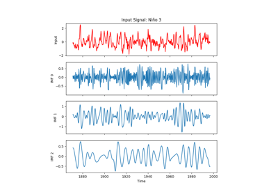
- easyclimate.filter.filter_emd(input_data: xarray.DataArray, time_step: Literal['ns', 'us', 'ms', 's', 'm', 'h', 'D', 'W', 'M', 'Y'], time_array=None, time_dim: str = 'time', spline_kind: Literal['cubic', 'akima', 'pchip', 'cubic_hermite', 'slinear', 'quadratic', 'linear'] = 'cubic', nbsym: int = 2, max_iteration: int = 1000, energy_ratio_thr: float = 0.2, std_thr: float = 0.2, svar_thr: float = 0.001, total_power_thr: float = 0.005, range_thr: float = 0.001, extrema_detection: Literal['simple', 'parabol'] = 'simple', max_imf: int = -1, dtype=np.float64)
Empirical Mode Decomposition
Method of decomposing signal into Intrinsic Mode Functions (IMFs) based on algorithm presented in Huang et al (1998).
Algorithm was validated with Rilling et al (2003). Matlab’s version from 3.2007.
Threshold which control the goodness of the decomposition:
std_thr: Test for the proto-IMF how variance changes between siftings.svar_thr: Test for the proto-IMF how energy changes between siftings.total_power_thr: Test for the whole decomp how much of energy is solved.range_thr: Test for the whole decomp whether the difference is tiny.
Parameters
- input_data:
xarray.DataArray Input signal data to be decomposed.
- time_step:
str Time step unit for datetime conversion (e.g., ‘s’, ‘ms’, ‘us’, ‘ns’).
- time_array:
array-like, optional Custom time array for the input signal. If None, uses input_data’s time dimension.
- time_dim:
str, default: time. The time coordinate dimension name.
- spline_kind:
Literal["cubic", "akima", "pchip", "cubic_hermite", "slinear", "quadratic", "linear"], default: “cubic” Type of spline used for envelope interpolation.
- nbsym:
int, default: 2 Number of points to add at signal boundaries for mirroring.
- max_iteration:
int, default: 1000 Maximum number of iterations per single sifting in EMD.
- energy_ratio_thr:
float, default: 0.2 Threshold value on energy ratio per IMF check.
- std_thr:
float, default: 0.2 Threshold value on standard deviation per IMF check.
- svar_thr:
float, default: 0.001 Threshold value on scaled variance per IMF check.
- total_power_thr:
float, default: 0.005 Threshold value on total power per EMD decomposition.
- range_thr:
float, default: 0.001 Threshold for amplitude range (after scaling) per EMD decomposition.
- extrema_detection:
Literal["simple", "parabol"], default: “simple” Method used to finding extrema.
- max_imf:
int, default: -1 IMF number to which decomposition should be performed. Negative value means all.
- dtype:
numpy.dtype, default: np.float64 Data type used for calculations.
Reference
Huang Norden E., Shen Zheng, Long Steven R., Wu Manli C., Shih Hsing H., Zheng Quanan, Yen Nai-Chyuan, Tung Chi Chao and Liu Henry H. 1998 The empirical mode decomposition and the Hilbert spectrum for nonlinear and non-stationary time series analysisProc. R. Soc. Lond. A.454903–995 http://doi.org/10.1098/rspa.1998.0193
Gabriel Rilling, Patrick Flandrin, Paulo Gonçalves. On empirical mode decomposition and its algorithms. IEEE-EURASIP Workshop on Nonlinear Signal and Image Processing NSIP-03, Jun 2003, Grado, Italy. https://inria.hal.science/inria-00570628v1
Colominas, M. A., Schlotthauer, G., and Torres, M. E. (2014). Improved complete ensemble EMD: A suitable tool for biomedical signal processing. Biomedical Signal Processing and Control, 14, 19-29. https://doi.org/10.1016/j.bspc.2014.06.009
Hsuan, R. (2014). Ensemble Empirical Mode Decomposition Parameters Optimization for Spectral Distance Measurement in Hyperspectral Remote Sensing Data. Remote Sens. 6(3), 2069-2083. http://doi.org/10.3390/rs6032069. http://www.mdpi.com/2072-4292/6/3/2069
Kim, D., and HS. Uh (2009). EMD: A Package for Empirical Mode Decomposition and Hilbert Spectrum. https://journal.r-project.org/archive/2009-1/RJournal_2009-1_Kim+Oh.pdf
Lambert et al. Empirical Mode Decomposition. https://www.clear.rice.edu/elec301/Projects02/empiricalMode/
Meta Trader. Introduction to the Empirical Mode Decomposition Method. https://www.mql5.com/en/articles/439
Salisbury, J.I. and Wimbush, M. (2002). Using modern time series analysis techniques to predict ENSO events from the SOI time series. Nonlinear Processes in Geophysics, 9, 341-345. http://www.nonlin-processes-geophys.net/9/341/2002/npg-9-341-2002.pdf
Torres, M. E., Colominas, M. A., Schlotthauer, G., & Flandrin, P. (2011). A complete ensemble empirical mode decomposition with adaptive noise. ICASSP, 4144-4147. http://doi.org/10.1109/ICASSP.2011.5947265.
Wang, T., M. Zhang, Q. Yu, and H. Zhang (2012). Comparing the applications of EMD and EEMD on time-frequency analysis of seismic signal. J. Appl. Geophys., 83, 29-34. http://doi.org/10.1016/j.jappgeo.2012.05.002.
Wu, Z., & Huang, N. E. (2009). Ensemble empirical mode decomposition: a noise-assisted data analysis method. Advances in Adaptive Data Analysis, 01(01), 1-41. https://doi.org/10.1142/S1793536909000047
Wu, Z, et al (2015). Fast multidimensional ensemble empirical mode decomposition for the analysis of big spatio-temporal datasets. Philos Trans A Math Phys Eng Sci, 374(2065), 20150197. http://doi.org/10.1098/rsta.2015.0197. https://www.ncbi.nlm.nih.gov/pmc/articles/PMC4792406/
Wu, Y. and Shen, BW (2016). An Evaluation of the Parallel Ensemble Empirical Mode Decomposition Method in Revealing the Role of Downscaling Processes Associated with African Easterly Waves in Tropical Cyclone Genesis. http://doi.org/10.1175/JTECH-D-15-0257.1. http://journals.ametsoc.org/doi/abs/10.1175/JTECH-D-15-0257.1
Empirical Mode Decomposition (EMD) and Ensemble Empirical Mode Decomposition (EEMD)
Empirical Mode Decomposition (EMD) and Ensemble Empirical Mode Decomposition (EEMD)
- easyclimate.filter.filter_eemd(input_data: xarray.DataArray, time_step, time_array=None, time_dim: str = 'time', noise_seed: None | int = None, trials: int = 100, noise_width: float = 0.05, parallel: bool = False, processes: None | int = None, separate_trends: bool = False, spline_kind: Literal['cubic', 'akima', 'pchip', 'cubic_hermite', 'slinear', 'quadratic', 'linear'] = 'cubic', nbsym: int = 2, max_iteration: int = 1000, energy_ratio_thr: float = 0.2, std_thr: float = 0.2, svar_thr: float = 0.001, total_power_thr: float = 0.005, range_thr: float = 0.001, extrema_detection: Literal['simple', 'parabol'] = 'parabol', dtype=np.float64)
Ensemble Empirical Mode Decomposition (EEMD)
Ensemble empirical mode decomposition (EEMD) is noise-assisted technique (Wu & Huang, 2009), which is meant to be more robust than simple Empirical Mode Decomposition (EMD). The robustness is checked by performing many decompositions on signals slightly perturbed from their initial position. In the grand average over all IMF results the noise will cancel each other out and the result is pure decomposition.
Parameters
- input_data:
xarray.DataArray Input signal data to be decomposed.
- time_step:
str Time step unit for datetime conversion (e.g., ‘s’, ‘ms’, ‘us’, ‘ns’).
- time_array:
array-like, optional Custom time array for the input signal. If None, uses input_data’s time dimension.
- time_dim:
str, default: “time” The time coordinate dimension name.
- noise_seed:
intor None, default: None Set seed for noise generation.
Warning
Given the nature of EEMD, each time you decompose a signal you will obtain a different set of components. That’s the expected consequence of adding noise which is going to be random. To make the decomposition reproducible, one needs to set a seed for the random number generator used in EEMD.
- trials:
int, default: 100 Number of trials or EMD performance with added noise.
- noise_width:
float, default: 0.05 Standard deviation of Gaussian noise (\(\hat\sigma\)). It’s relative to absolute amplitude of the signal, i.e. \(\hat\sigma = \sigma\cdot|\max(S)-\min(S)|\), where \(\sigma\) is noise_width.
- parallel:
bool, default: False Flag whether to use multiprocessing in EEMD execution. Since each EMD(s+noise) is independent this should improve execution speed considerably. Note that it’s disabled by default because it’s the most common problem when EEMD takes too long time to finish. If you set the flag to True, make also sure to set processes to some reasonable value.
- processes:
intor None, default: None Number of processes harness when executing in parallel mode. The value should be between 1 and max that depends on your hardware. If None, uses all available cores.
- separate_trends:
bool, default: False Flag whether to isolate trends from each EMD decomposition into a separate component. If
True, the resulting EEMD will contain ensemble only from IMFs and the mean residue will be stacked as the last element.- spline_kind:
Literal["cubic", "akima", "pchip", "cubic_hermite", "slinear", "quadratic", "linear"], default: “cubic” Type of spline used for envelope interpolation.
- nbsym:
int, default: 2 Number of points to add at signal boundaries for mirroring.
- max_iteration:
int, default: 1000 Maximum number of iterations per single sifting in EMD.
- energy_ratio_thr:
float, default: 0.2 Threshold value on energy ratio per IMF check.
- std_thr:
float, default: 0.2 Threshold value on standard deviation per IMF check.
- svar_thr:
float, default: 0.001 Threshold value on scaled variance per IMF check.
- total_power_thr:
float, default: 0.005 Threshold value on total power per EMD decomposition.
- range_thr:
float, default: 0.001 Threshold for amplitude range (after scaling) per EMD decomposition.
- extrema_detection:
Literal["simple", "parabol"], default: “parabol” Method used to finding extrema.
- dtype:
numpy.dtype, default: np.float64 Data type used for calculations.
Returns
xarray.DatasetDataset containing the input data and the decomposed eIMFs (Ensemble IMFs).
Reference
Wu, Z., & Huang, N. E. (2009). Ensemble empirical mode decomposition: a noise-assisted data analysis method. Advances in Adaptive Data Analysis, 01(01), 1-41. https://doi.org/10.1142/S1793536909000047
See also
filter_emd(): Standard Empirical Mode Decomposition
Empirical Mode Decomposition (EMD) and Ensemble Empirical Mode Decomposition (EEMD)
Empirical Mode Decomposition (EMD) and Ensemble Empirical Mode Decomposition (EEMD)- input_data:
- easyclimate.filter.calc_gaussian_filter(data: xarray.DataArray, window_length: float, sigma: float = None, dim: str = 'time', keep_attrs: bool = False) xarray.DataArray
Apply a Gaussian filter to data along a specified dimension.
Parameters
- da
xarray.DataArray Input data array
- window_length:
int, optional The window width.
- sigma
float, optional Standard deviation for Gaussian kernel. If None, calculated as \(\mathrm{window_length} / \sqrt{8 log2}\).
- dim
str, optional Dimension along which to filter (default: ‘time’)
- keep_attrs
bool, optional Whether to preserve attributes (default: False)
Returns
xarray.DataArraySmoothed data with the same dimensions as input.
- da

- easyclimate.filter.calc_time_spectrum(data: xarray.DataArray, time_dim: str = 'time', inv: bool = False) tuple[xarray.DataArray, xarray.DataArray]
Calculate the time spectrum of a multi-dimensional
xarray.DataArrayalong the time dimension.Parameters
- data
xarray.DataArray Input data with at least a time dimension.
- time_dim
str, optional Name of the time dimension in the DataArray, by default
'time'- inv
bool, optional If True, use forward FFT instead of inverse, by default
False
Returns
easyclimate.DataNode, containing:Amplitude spectrum (same dimensions as input but with
freqandperioddimension)Frequency or period values
Tip
The function automatically handles even/odd length time series and removes the zero-frequency component. The amplitude is calculated as the power spectrum (\(|\mathrm{fft}|^2\)).
- data
- easyclimate.filter.calc_mean_fourier_amplitude(data: xarray.DataArray, time_dim: str = 'time', lower: float = None, upper: float = None) xarray.DataArray
Calculate mean Fourier amplitude between specified period bounds.
Parameters
- data
xarray.DataArray Input data with at least a time dimension. Can have additional dimensions.
- time_dim
str, optional Name of the time coordinate in the DataArray, by default
'time'- lower
float Lower bound of period range
- upper
float Upper bound of period range
Returns
xarray.DataArrayMean amplitude within specified period range, with same dimensions as input but without time dimension.
Tip
The bounds should be in the same units as returned by
easyclimate.filter.spectrum.calc_time_spectrumUses
easyclimate.filter.spectrum.calc_time_spectruminternallyThe amplitude is scaled by the variance of the input data
- data
- easyclimate.filter.filter_fourier_harmonic_analysis(da: xarray.DataArray, time_dim: str = 'time', period_bounds: tuple = (None, None), filter_type: Literal['highpass', 'lowpass', 'bandpass'] = 'bandpass', sampling_interval: float = 1.0, apply_window: bool = True) xarray.DataArray
Apply Fourier harmonic analysis to filter an dataset along a time dimension.
Parameters
- da
xarray.DataArray Input data array with a time dimension (e.g., z200 with dims [time, lat, lon]).
- time_dim
str, optional Name of the time dimension (default: ‘time’).
- period_bounds
tuple, optional Period range for filtering in units of sampling_interval (e.g., years if sampling_interval=1). Format:
(min_period, max_period). Use None for unbounded limits.High-pass:
(None, max_period)to retain periods < max_period.Low-pass:
(min_period, None)to retain periods > min_period.Bandpass:
(min_period, max_period)to retain min_period < periods < max_period.
- filter_type
str, optional Type of filter:
'highpass','lowpass', or'bandpass'(default:'bandpass').- sampling_interval
float, optional Sampling interval of the time dimension (default: 1.0, e.g., 1 year for annual data).
- apply_window
bool, optional Apply a Hann window to reduce boundary effects (default: True).
Returns
xarray.DataArrayFiltered data array with same dimensions and coordinates as input.
Examples
>>> # Create example data
>>> ds = xr.DataArray(
...    np.random.randn(56, 90, 180),
...    dims=['time', 'lat', 'lon'],
...    coords={
...        'time': np.arange(1948, 2004),
...        'lat': np.linspace(-90, 90, 90),
...        'lon': np.linspace(0, 360, 180, endpoint=False)
...    },
...    name='z200'
... )
>>> # Apply low-pass filter to retain periods > 8 years
>>> ds_filtered = filter_fourier_harmonic_analysis(
...    da=ds,
...    time_dim='time',
...    period_bounds=(8.0, None),
...    filter_type='lowpass',
...    sampling_interval=1.0,
...    apply_window=True
... )
- da
- easyclimate.filter.mask_custom_rectangular_box(da: xarray.DataArray, lon1: float, lon2: float, lat1: float, lat2: float, angle: float = 0.0, center: Literal['center', 'lowerleft'] = 'center', use_coslat: bool = True, lat_dim: str = 'lat', lon_dim: str = 'lon')
Generate a mask for a custom geographical rectangular box with optional rotation.
Parameters
- da
xarray.DataArray Input data array containing latitude and longitude coordinates. The mask is generated on the horizontal grid defined by lat_dim and lon_dim.
- lon1, lon2:
float. Rectangular box longitude point. The applicable value should be between -180 \(^\circ\) and 360 \(^\circ\). lon1 and lon2 are used to define the unrotated box extent, and do not strictly require the size relationship between them.
- lat1, lat2:
float. Rectangular box latitude point. The applicable value should be between -90 \(^\circ\) and 90 \(^\circ\). lat1 and lat2 are used to define the unrotated box extent, and do not strictly require the size relationship between them.
- angle:
float, default: 0.0. Counterclockwise rotation angle in degrees.
- center:
str, default: “center”. Rotation pivot of the rectangular box.
“center”: rotate around the box center.
“lowerleft”: rotate around the lower-left corner of the box.
- use_coslat:
bool, default: True. Whether to apply local geographical metric correction before rotation. If True, longitude is scaled by \(\cos(lat0)\) using the selected pivot latitude so that longitude and latitude have a locally comparable distance scale.
- lat_dim:
str, default: “lat”. Name of the latitude coordinate in da.
- lon_dim:
str, default: “lon”. Name of the longitude coordinate in da.
Returns
- mask
xarray.DataArray Boolean mask on the same horizontal grid as da, where values are True inside the rotated rectangular box and False outside.
- da