easyclimate.field.typhoon
Submodules
Functions
Calculate potential intensity of TC (tropical cyclone) according to the Bister and Emanuel (2002) algorithm. |
|
|
Tracks the center of a cyclone using biquadratic interpolation on mean sea level pressure (MSL) data. |
|
Performs axisymmetric analysis of a cyclone by transforming data into a polar coordinate system centered on the cyclone. |
Package Contents
- easyclimate.field.typhoon.calc_potential_intensity_Bister_Emanuel_2002(sst_data: xarray.DataArray, sst_data_units: Literal['celsius', 'kelvin', 'fahrenheit'], surface_pressure_data: xarray.DataArray, surface_pressure_data_units: Literal['hPa', 'Pa', 'mbar'], temperature_data: xarray.DataArray, temperature_data_units: Literal['celsius', 'kelvin', 'fahrenheit'], specific_humidity_data: xarray.DataArray, specific_humidity_data_units: Literal['kg/kg', 'g/kg', 'g/g'], vertical_dim: str, vertical_dim_units: Literal['hPa', 'Pa', 'mbar'], CKCD: float = 0.9, ascent_flag: bool = False, diss_flag: bool = True, V_reduc: float = 0.8, ptop: float = 50, miss_handle: bool = True) xarray.Dataset
Calculate potential intensity of TC (tropical cyclone) according to the Bister and Emanuel (2002) algorithm.
This function calculates the maximum wind speed and mimimum central pressure achievable in tropical cyclones, given a sounding and a sea surface temperature.
From Bister and Emanuel (1998) EQN. 21, PI may be computed directly via:
\[V_{max}^{2} = \frac{C_k}{C_D}(\frac{T_{s} - T_{0}}{T_{0}})(h_0^* - h^*),\]where \(C_k\) and \(C_D\) are the enthalpy and momentum surface exchange coefficients, respectively; \(T_{s}\) is the sea surface temperature; \(T_{0}\) is the mean outflow temperature; \(h_0^*\) is the saturation moist static energy at the sea surface; and \(h^*\) is the moist static energy of the free troposphere. The ratio \(\frac{C_k}{C_D}\) is an uncertain quantity typically taken to be a constant (default is 0.9, see Emanuel 2003 and references therein).
Building on this definition, one can extract TC efficiency and disequilibrium, and decompose the terms to determine their relative contributions to potential intensity.
The efficiency of TC PI is the Carnot efficiency. Typical values range between 50-70% in the tropics.
Each term in the PI equation may decomposed by taking the natural logarithm of both sides, arriving at (Wing et al. 2015; EQN. 2):
\[2*\log(V_{max}) = \log(\frac{C_k}{C_D}) + \log(\frac{T_{s} - T_{0}}{T_{0}}) + \log(h_0^* - h^*).\]Note that the units of everything input to the functions (and particularly the temperatures) must match.
Parameters
- sst_data:
xarray.DataArray. The sea surface temperature data.
- sst_data_units:
str. The unit corresponding to sst_data value. Optional values are celsius, kelvin, fahrenheit.
- surface_pressure_data:
xarray.DataArray. Mean surface sea level pressure.
- surface_pressure_data_units:
str. The unit corresponding to surface_pressure_data value. Optional values are hPa, Pa, mbar.
- temperature_data:
xarray.DataArray. Atmospheric temperature.
- temperature_data_units:
str. The unit corresponding to temperature_data value. Optional values are celsius, kelvin, fahrenheit.
- specific_humidity_data:
xarray.DataArray. The Specific humidity of air.
- specific_humidity_data_units:
str. The unit corresponding to specific_humidity value. Optional values are kg/kg, g/g, g/kg and so on.
- vertical_dim:
str. Vertical coordinate dimension name.
- vertical_dim_units:
str. The unit corresponding to the vertical p-coordinate value. Optional values are hPa, Pa, mbar.
- CKCD:
float, default 0.9. Ratio of \(C_k\) to \(C_D\) (unitless number), i.e. the ratio of the exchange coefficients of enthalpy and momentum flux (e.g. see Bister and Emanuel 1998, EQN. 17-18). More discussion on \(\frac{C_k}{C_D}\) is found in Emanuel (2003). Default is 0.9 based on e.g. Wing et al. (2015).
- ascent_flag:
bool, default False. Adjustable constant fraction (unitless fraction) for buoyancy of displaced parcels, where True is Reversible ascent (default) and False is Pseudo-adiabatic ascent.
- V_reduc:
float, default 0.8. Adjustable constant fraction (unitless fraction) for reduction of gradient winds to 10-m winds see Emanuel (2000) and Powell (1980).
- ptop:
float, default 50 hPa. Pressure below which sounding is ignored (hPa).
- miss_handle:
bool, default True. Flag that determines how missing (NaN) values are handled in CAPE calculation. - If False (BE02 default), NaN values in profile are ignored and PI is still calcuated. - If True, given NaN values PI will be set to missing (with IFLAG=3 in CAPE calculation).
Note
If any missing values are between the lowest valid level and ptop then PI will automatically be set to missing (with IFLAG=3 in CAPE calculation)
Returns
vmax: The maximum surface wind speed (m/s) reduced to reflect surface drag via \(V_{\text{reduc}}\).
pmin: The minimum central pressure (hPa)
ifl: A flag value: A value of 1 means OK; a value of 0 indicates no convergence; a value of 2 means that the CAPE routine failed to converge; a value of 3 means the CAPE routine failed due to missing data in the inputs.
t0: The outflow temperature (K)
otl: The outflow temperature level (hPa), defined as the level of neutral bouyancy where the outflow temperature is found, i.e. where buoyancy is actually equal to zero under the condition of an air parcel that is saturated at sea level pressure.
eff: Tropical cyclone efficiency.
diseq: Thermodynamic disequilibrium.
lnpi: Natural \(\log(\text{Potential Intensity})\)
lneff: Natural \(\log(\text{Tropical Cyclone Efficiency})\)
lndiseq: Natural \(\log(\text{Thermodynamic Disequilibrium})\)
lnCKCD: Natural \(\log(C_k/C_D)\)
Reference
Bister, M., Emanuel, K.A. Dissipative heating and hurricane intensity. Meteorl. Atmos. Phys. 65, 233–240 (1998). https://doi.org/10.1007/BF01030791
Bister, M., and K. A. Emanuel, Low frequency variability of tropical cyclone potential intensity, 1, Interannual to interdecadal variability, J. Geophys. Res., 107(D24), 4801, https://doi.org/10.1029/2001JD000776, 2002.
Emanuel, K.: A Statistical Analysis of Tropical Cyclone Intensity, Mon. Weather Rev., 128, 1139–1152, https://doi.org/10.1175/1520-0493(2000)128<1139:ASAOTC>2.0.CO;2, 2000.
Emanuel, K.: Tropical Cyclones, Annu. Rev. Earth Pl. Sc., 31, 75–104, https://doi.org/10.1146/annurev.earth.31.100901.141259, 2003.
Gilford, D. M.: pyPI (v1.3): Tropical Cyclone Potential Intensity Calculations in Python, Geosci. Model Dev., 14, 2351–2369, https://doi.org/10.5194/gmd-14-2351-2021, 2021.
Powell, M. D.: Evaluations of Diagnostic Marine Boundary-Layer Models Applied to Hurricanes, Mon. Weather Rev., 108, 757–766, https://doi.org/10.1175/1520-0493(1980)108<0757:EODMBL>2.0.CO;2, 1980.
Wing, A. A., Emanuel, K., and Solomon, S.: On the factors affecting trends and variability in tropical cyclone potential intensity, Geophys. Res. Lett., 42, 8669–8677, https://doi.org/10.1002/2015GL066145, 2015.
- sst_data:

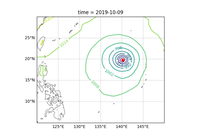
- easyclimate.field.typhoon.track_cyclone_center_msl_only(msl_data: xarray.DataArray, sample_point: Tuple[float, float], index_value: List[int] | List[float] = [0], lon_dim: str = 'lon', lat_dim: str = 'lat') pandas.DataFrame
Tracks the center of a cyclone using biquadratic interpolation on mean sea level pressure (MSL) data.
This function identifies local minima in the MSL data using a minimum filter with cyclic boundary conditions in longitude, selects the minimum closest to the provided sample point in geodesic distance, and applies biquadratic interpolation to estimate the precise location of the cyclone center. If interpolation fails, the grid-based minimum is used.
This is a simple approach used by the author in pytrack to identify local minima in sea-level pressure.
Local minima are identified using
scipy.ndimage.minimum_filter(). To ensure consistency with the subsequent quadratic interpolation, we search for minima within a \(3 \\cdot 3\) grid. Since the region is cropped, themodeparameter is set tonearest, which extends the boundary values for both latitude and longitude dimensions.Given an estimated position, e.g., \(\\lambda = 140^\\circ, \\phi = 20^\\circ\) in
sample_point, we calculate the great-circle distance \(d = a\\alpha\) (\(a\) is the Earth’s radius) to the identified local minima using the formula:\[\begin{split}\\cos \\alpha = \\sin\\theta_0 \\sin\\theta + \\cos\\theta_0 \\cos\\theta \\cos(\\lambda - \\lambda_0).\end{split}\]Since the relative magnitude remains unchanged when comparing the central angle \(\\alpha\) on a unit sphere, the Earth’s radius is omitted.
The location of the local minima closest to the given longitude and latitude is identified. This point and its eight neighboring points, totaling nine points, are stored in a one-dimensional array. The center is indexed as 0, and the points are stored counterclockwise starting from the bottom-left corner.
Let \(f\) be a quadratic function of \(x\) and \(y\):
\[f(x, y) = c_0 + c_1x + c_2y + c_3xy + c_4x^2 + c_5y^2 + c_6x^2y + c_7xy^2 + c_8x^2y^2.\]A necessary condition for the quadratic function to have an extremum is that its gradient is zero. At grid points, assume \(f(x_0, y_0)\) is a local minimum. The extremum of \(f(x, y)\) may not necessarily lie on a grid point. Suppose the extremum of \(f(x, y)\) is at \(x_0 + \\Delta x, y_0 + \\Delta y\). Expanding around \(x_0, y_0\) using a Taylor series gives:
\[\begin{split}f(x, y) = f(x_0, y_0) + f_x\\Delta x + f_y\\Delta y + \\frac{1}{2}f_{xx}(\\Delta x)^2 + \\frac{1}{2}f_{yy}(\\Delta y)^2 + f_{xy}\\Delta x\\Delta y.\end{split}\]Define:
\[\begin{split}\\begin{align} \\mathbf{b} &= -\\begin{bmatrix} f_x \\ f_y \\end{bmatrix}, \\\\ \\mathbf{A} &= \\begin{bmatrix} f_{xx} & f_{xy} \\\ f_{xy} & f_{yy} \\end{bmatrix}, \\\\ \\mathbf{x} &= \\begin{bmatrix} \\Delta x \\\ \\Delta y \\end{bmatrix}. \\end{align}\end{split}\]Then:
\[\begin{split}\\begin{align} f(x, y) &= f(x_0, y_0) - \\mathbf{b}^T\\mathbf{x} + \\frac{1}{2}\\mathbf{x}^T\\mathbf{A}\\mathbf{x}, \\\\ \\nabla f &= \\mathbf{A}\\mathbf{x} - \\mathbf{b} = 0, \\\\ \\mathbf{x} &= \\mathbf{A}^{-1}\\mathbf{b}. \\end{align}\end{split}\]When \(d \\equiv f_{xx}f_{yy} - f_{xy}^2 \\ne 0\):
\[\begin{split}\\mathbf{A}^{-1} = \\frac{1}{d} \\begin{pmatrix} f_{yy} & -f_{xy} \\\ -f_{xy} & f_{xx} \\end{pmatrix},\end{split}\]allowing \(\\Delta x\) and \(\\Delta y\) to be determined, thus locating the extremum.
Parameters
- msl_data
xarray.DataArray Input mean sea level pressure data with latitude and longitude dimensions.
- sample_point
tuple[float, float] Initial guess for the cyclone center as (longitude, latitude) in degrees.
- index_value
List[int] | List[float], optional Index value(s) for the output DataFrame, default is [0].
- lon_dim
str, optional Name of the longitude dimension, default is ‘lon’.
- lat_dim
str, optional Name of the latitude dimension, default is ‘lat’.
Returns
pandas.DataFrameDataFrame containing the longitude, latitude, and minimum MSL pressure of the cyclone center.
Example
>>> import xarray as xr
>>> import numpy as np
>>> slp = xr.DataArray(np.random.rand(20, 30), dims=['lat', 'lon'],
...                    coords={'lat': np.linspace(-10, 10, 20), 'lon': np.linspace(100, 130, 30)})
>>> result = track_cyclone_center_msl_only(slp, (110, 0), index_value = [0])
- msl_data
- easyclimate.field.typhoon.cyclone_axisymmetric_analysis(data_input: xarray.DataArray, cyclone_center_point: Tuple[float, float], polar_lon: numpy.ndarray = np.arange(0, 360, 2), polar_lat: numpy.ndarray = np.arange(80, 90.1, 1), lon_dim: str = 'lon', lat_dim: str = 'lat', vertical_dim: str = 'level', R: float = 6371.0087714) easyclimate.core.datanode.DataNode
Performs axisymmetric analysis of a cyclone by transforming data into a polar coordinate system centered on the cyclone.
This function converts input data to a polar coordinate system based on the cyclone center, interpolates the data onto a polar grid, and decomposes it into symmetric and asymmetric components. The symmetric component is the azimuthal mean, and the asymmetric component is the deviation from this mean.
Parameters
- data_input
xarray.DataArray Input data with latitude, longitude, and optionally vertical dimensions, i.e.,
(lat, lon)or(level, lat, lon).- cyclone_center_pointTuple[float, float]
Cyclone center as
(longitude, latitude)in degrees.- polar_lon
numpy.ndarray, optional Array of longitudinal angles in degrees for the polar grid, default is
np.arange(0, 360, 2).- polar_lat
numpy.ndarray, optional Array of latitudinal angles in degrees for the polar grid, default is
np.arange(80, 90.1, 1).- lon_dim
str, optional Name of the longitude dimension, default is ‘lon’.
- lat_dim
str, optional Name of the latitude dimension, default is ‘lat’.
- vertical_dim
str, optional Name of the vertical dimension, default is ‘level’.
- R
float, optional ( \(\mathrm{km}\) ). Earth’s radius, default is 6371.0087714.
Returns
easyclimate.DataNodeA DataNode containing three xarray.DataArray objects:
rotated: Data interpolated onto the polar grid.
rotated_symmetric: Azimuthal mean of the rotated data.
rotated_asymmetric: Deviation from the azimuthal mean.
See also
https://www.dpac.dpri.kyoto-u.ac.jp/enomoto/pymetds/Typhoon.html
Enomoto, T. (榎本 剛) (2019). Influence of the Track Forecast of Typhoon Prapiroon on the Heavy Rainfall in Western Japan in July 2018. SOLA, 15A, 66-71. https://doi.org/10.2151/sola.15A-012
Nakashita, S. (中下 早織), & Enomoto, T. (2021). Factors for an Abrupt Increase in Track Forecast Error of Typhoon Hagibis (2019). SOLA, 17A(Special_Edition), 33-37. https://doi.org/10.2151/sola.17A-006
Example
>>> import xarray as xr
>>> import numpy as np
>>> data = xr.DataArray(np.random.rand(37, 241, 241), dims=['level', 'lat', 'lon'],
...                     coords={'level': np.array([1, 2, 3, 5, 7, 10, 20, 30, 50, 70, 100, 125, 150, 175, 200, 225, 250, 300, 350, 400, 450, 500, 550, 600, 650, 700, 750, 775, 800, 825, 850, 875, 900, 925, 950, 975, 1000]),
...                             'lat': np.arange(60, 0-0.25, -0.25),
...                             'lon': np.arange(110, 170 + 0.25, 0.25)
... )
>>> result = cyclone_axisymmetric_analysis(data, (140.20, 19.77))
>>> print(result)
<easyclimate.DataNode 'root'>
root: /
├── rotated: <xarray.DataArray>
│   Dimensions:  (level: 37, y: 11, polar_lon: 180)
│   Coordinates:
│     * lat        (y: 11): float64
│     * level      (level: 37): int32
│     * lon        (polar_lon: 180): int64
│     * polar_lat  (y: 11): float64
│     * polar_lon  (polar_lon: 180): int64
│     * y          (y: 11): float64
├── rotated_asymmetric: <xarray.DataArray>
│   Dimensions:  (level: 37, y: 11, polar_lon: 180)
│   Coordinates:
│     * lat        (y: 11): float64
│     * level      (level: 37): int32
│     * lon        (polar_lon: 180): int64
│     * polar_lat  (y: 11): float64
│     * polar_lon  (polar_lon: 180): int64
│     * y          (y: 11): float64
└── rotated_symmetric: <xarray.DataArray>
    Dimensions:  (level: 37, y: 11)
    Coordinates:
    * lat        (y: 11): float64
    * level      (level: 37): int32
    * polar_lat  (y: 11): float64
    * y          (y: 11): float64
- data_input