easyclimate.field.teleconnection
Submodules
- easyclimate.field.teleconnection.index_ao_nam
- easyclimate.field.teleconnection.index_bbo
- easyclimate.field.teleconnection.index_cgt
- easyclimate.field.teleconnection.index_da
- easyclimate.field.teleconnection.index_ea
- easyclimate.field.teleconnection.index_eu
- easyclimate.field.teleconnection.index_nao
- easyclimate.field.teleconnection.index_pna
- easyclimate.field.teleconnection.index_srp
- easyclimate.field.teleconnection.index_wa
- easyclimate.field.teleconnection.index_wp
Functions
|
The calculation of monthly mean PNA index is constructed by following modified pointwise method: |
|
The calculation of monthly mean PNA index using Pointwise method following Wallace and Gutzler (1981): |
|
The calculation of monthly mean PNA index using rotated empirical orthogonal functions (REOFs) method over the entire Northern Hemisphere: |
|
The calculation of monthly mean NAO index using rotated empirical orthogonal functions (REOFs) method: |
|
The calculation of monthly mean eastern Atlantic (EA) index using Pointwise method following Wallace and Gutzler (1981): |
|
The calculation of monthly mean western Atlantic (WA) index using Pointwise method following Wallace and Gutzler (1981): |
|
The calculation of monthly mean western Pacific (WP) index using Pointwise method following Wallace and Gutzler (1981): |
|
The calculation of monthly mean Eurasian pattern (EU) index using Pointwise method following Wallace and Gutzler (1981): |
|
The calculation of monthly mean SRP index using empirical orthogonal functions (EOFs) method based on Yasui and Watanabe (2010): |
|
The calculation of monthly mean SRP index using empirical orthogonal functions (EOFs) method based on Kosaka et al. (2009): |
|
The calculation of monthly mean SRP index using empirical orthogonal functions (EOFs) method based on Chen and Huang (2009): |
|
The calculation of monthly mean SRP index using empirical orthogonal functions (EOFs) method based on Sato and Takahashi (2006): |
|
The calculation of monthly mean SRP index based on Lu et al. (2002): |
|
The calculation of monthly mean circumglobal teleconnection pattern (CGT) index is constructed by following method: |
|
The calculation of monthly mean circumglobal teleconnection pattern (CGT) index using Ding, Q., & Wang, B. (2005) method |
|
The calculation of monthly mean Arctic Oscillation (AO) index using empirical orthogonal functions (EOFs) method over the entire Northern Hemisphere: |
|
The calculation of Monthly Northern Hemisphere Annular Mode (NAM) Index using normalized monthly zonal-mean sea level pressure (SLP) between 35°N and 65°N. |
|
The calculation of monthly mean Barents-Beaufort Oscillation (BBO) index using empirical orthogonal functions (EOFs) method |
|
The calculation of monthly mean Arctic Dipole Anomaly (DA/AD) index using empirical orthogonal functions (EOFs) method |
Package Contents
- easyclimate.field.teleconnection.calc_index_PNA_modified_pointwise(z_monthly_data: xarray.DataArray, time_range: slice = slice(None, None), lon_dim: str = 'lon', lat_dim: str = 'lat', time_dim: str = 'time', normalized: bool = True) xarray.DataArray
The calculation of monthly mean PNA index is constructed by following modified pointwise method:
\[\mathrm{PNA = Z^*(15^{\circ}N-25^{\circ}N,180-140^{\circ}W)-Z^*(40^{\circ}N-50^{\circ}N,180-140^{\circ}W)+Z^*(45^{\circ}N-60^{\circ}N,125^{\circ}W-105^{\circ}W)-Z^*(25^{\circ}N-35^{\circ}N,90^{\circ}W-70^{\circ}W)}\]where \(Z^*\) denotes monthly mean 500 hPa height anomaly.
Parameters
- z_monthly_data:
xarray.DataArray. The monthly geopotential height. The 500hPa layer is recommended.
- time_range:
slice, default: slice(None, None). The time range of seasonal cycle means to be calculated. The default value is the entire time range.
- lon_dim:
str, default: lon. Longitude coordinate dimension name. By default extracting is applied over the lon dimension.
- lat_dim:
str, default: lat. Latitude coordinate dimension name. By default extracting is applied over the lat dimension.
- time_dim:
str, default: time. The time coordinate dimension name.
- normalized:
bool, default True, optional. Whether to standardize the index based on standard deviation over time_range.
Returns
The monthly mean PNA index (
xarray.DataArray).Reference
- z_monthly_data:
- easyclimate.field.teleconnection.calc_index_PNA_Wallace_Gutzler_1981(z_monthly_data: xarray.DataArray, time_range: slice = slice(None, None), lon_dim: str = 'lon', lat_dim: str = 'lat', time_dim: str = 'time', normalized: bool = True) xarray.DataArray
The calculation of monthly mean PNA index using Pointwise method following Wallace and Gutzler (1981):
\[\mathrm{PNA = Z^*(20^{\circ}N,160^{\circ}W)-Z^*(45^{\circ}N,165^{\circ}W)+Z^*(55^{\circ}N,115^{\circ}W)-Z^*(30^{\circ}N,85^{\circ}W)}\]where \(Z^*\) denotes monthly mean 500 hPa height anomaly.
Parameters
- z_monthly_data:
xarray.DataArray. The monthly geopotential height. The 500hPa layer is recommended.
- time_range:
slice, default: slice(None, None). The time range of seasonal cycle means to be calculated. The default value is the entire time range.
- lon_dim:
str, default: lon. Longitude coordinate dimension name. By default extracting is applied over the lon dimension.
- lat_dim:
str, default: lat. Latitude coordinate dimension name. By default extracting is applied over the lat dimension.
- time_dim:
str, default: time. The time coordinate dimension name.
- normalized:
bool, default True, optional. Whether to standardize the index based on standard deviation over time_range.
Returns
The monthly mean PNA index (
xarray.DataArray).Reference
- z_monthly_data:
- easyclimate.field.teleconnection.calc_index_PNA_NH_REOF(z_monthly_data: xarray.DataArray, time_range: slice = slice(None, None), lon_dim: str = 'lon', lat_dim: str = 'lat', lat_range: slice = slice(20, 85), time_dim: str = 'time', random_state=None, solver: Literal['auto', 'full', 'randomized'] = 'auto', solver_kwargs: dict = {}, normalized: bool = True) xarray.DataArray
The calculation of monthly mean PNA index using rotated empirical orthogonal functions (REOFs) method over the entire Northern Hemisphere:
Parameters
- z_monthly_data:
xarray.DataArray. The monthly geopotential height. The 500hPa layer is recommended.
- time_range:
slice, default: slice(None, None). The time range of seasonal cycle means to be calculated. The default value is the entire time range.
- lon_dim:
str, default: lon. Longitude coordinate dimension name. By default extracting is applied over the lon dimension.
- lat_dim:
str, default: lat. Latitude coordinate dimension name. By default extracting is applied over the lat dimension.
- lat_range:
slice, default: slice(20, 85). The latitude range of computation using REOFs over the Northern Hemisphere. The default value is from \(\mathrm{20^{\circ}N}\) to \(\mathrm{85^{\circ}N}\).
- time_dim:
str, default: time. The time coordinate dimension name.
- random_state:
int, default None. Seed for the random number generator.
- solver: {“auto”, “full”, “randomized”}, default: “auto”.
Solver to use for the REOFs computation.
- solver_kwargs:
dict, default {}. Additional keyword arguments to be passed to the REOFs solver.
- normalized:
bool, default True, optional. Whether to standardize the index based on standard deviation over time_range.
Returns
The monthly mean PNA index (
xarray.DataArray).Reference
See also
- z_monthly_data:
- easyclimate.field.teleconnection.calc_index_NAO_NH_REOF(z_monthly_data: xarray.DataArray, time_range: slice = slice(None, None), lon_dim: str = 'lon', lat_dim: str = 'lat', lat_range: slice = slice(20, 85), time_dim: str = 'time', random_state: int | None = None, solver: Literal['auto', 'full', 'randomized'] = 'auto', solver_kwargs: dict = {}, normalized: bool = True) xarray.DataArray
The calculation of monthly mean NAO index using rotated empirical orthogonal functions (REOFs) method:
Parameters
- z_monthly_data:
xarray.DataArray. The monthly geopotential height.
- time_range:
slice, default: slice(None, None). The time range of seasonal cycle means to be calculated. The default value is the entire time range.
- lon_dim:
str, default: lon. Longitude coordinate dimension name. By default extracting is applied over the lon dimension.
- lat_dim:
str, default: lat. Latitude coordinate dimension name. By default extracting is applied over the lat dimension.
- lat_range:
slice, default: slice(20, 85). The latitude range of computation using REOFs over the Northern Hemisphere. The default value is from \(\mathrm{20^{\circ}N}\) to \(\mathrm{85^{\circ}N}\).
- time_dim:
str, default: time. The time coordinate dimension name.
- random_state:
int, default None. Seed for the random number generator.
- solver: {“auto”, “full”, “randomized”}, default: “auto”.
Solver to use for the SVD computation.
- solver_kwargs:
dict, default {}. Additional keyword arguments to be passed to the SVD solver.
- normalized:
bool, default True, optional. Whether to standardize the index based on standard deviation over time_range.
Returns
The monthly mean NAO index (
xarray.DataArray).Reference
See also
- z_monthly_data:
- easyclimate.field.teleconnection.calc_index_EA_Wallace_Gutzler_1981(z_monthly_data: xarray.DataArray, time_range: slice = slice(None, None), lon_dim: str = 'lon', lat_dim: str = 'lat', time_dim: str = 'time', normalized: bool = True) xarray.DataArray
The calculation of monthly mean eastern Atlantic (EA) index using Pointwise method following Wallace and Gutzler (1981):
\[\mathrm{EA = \frac{1}{2} Z^*(55^{\circ}N, 20^{\circ}W) - \frac{1}{4} Z^*(25^{\circ}N, 25^{\circ}W) - \frac{1}{4} Z^*(50^{\circ}N, 40^{\circ}E)}\]where \(Z^*\) denotes monthly mean 500 hPa height anomaly.
Parameters
- z_monthly_data:
xarray.DataArray. The monthly geopotential height. The 500hPa layer is recommended.
- time_range:
slice, default: slice(None, None). The time range of seasonal cycle means to be calculated. The default value is the entire time range.
- lon_dim:
str, default: lon. Longitude coordinate dimension name. By default extracting is applied over the lon dimension.
- lat_dim:
str, default: lat. Latitude coordinate dimension name. By default extracting is applied over the lat dimension.
- time_dim:
str, default: time. The time coordinate dimension name.
Returns
The monthly mean EA index (
xarray.DataArray).Reference
- z_monthly_data:
- easyclimate.field.teleconnection.calc_index_WA_Wallace_Gutzler_1981(z_monthly_data: xarray.DataArray, time_range: slice = slice(None, None), lon_dim: str = 'lon', lat_dim: str = 'lat', time_dim: str = 'time', normalized: bool = True) xarray.DataArray
The calculation of monthly mean western Atlantic (WA) index using Pointwise method following Wallace and Gutzler (1981):
\[\mathrm{WA = \frac{1}{2} [Z^*(55^{\circ}N, 55^{\circ}W) - Z^*(30^{\circ}N, 55^{\circ}W)] }\]where \(Z^*\) denotes monthly mean 500 hPa height anomaly.
Parameters
- z_monthly_data:
xarray.DataArray. The monthly geopotential height. The 500hPa layer is recommended.
- time_range:
slice, default: slice(None, None). The time range of seasonal cycle means to be calculated. The default value is the entire time range.
- lon_dim:
str, default: lon. Longitude coordinate dimension name. By default extracting is applied over the lon dimension.
- lat_dim:
str, default: lat. Latitude coordinate dimension name. By default extracting is applied over the lat dimension.
- time_dim:
str, default: time. The time coordinate dimension name.
- normalized:
bool, default True, optional. Whether to standardize the index based on standard deviation over time_range.
Returns
The monthly mean WA index (
xarray.DataArray).Reference
- z_monthly_data:
- easyclimate.field.teleconnection.calc_index_WP_Wallace_Gutzler_1981(z_monthly_data: xarray.DataArray, time_range: slice = slice(None, None), lon_dim: str = 'lon', lat_dim: str = 'lat', time_dim: str = 'time', normalized: bool = True) xarray.DataArray
The calculation of monthly mean western Pacific (WP) index using Pointwise method following Wallace and Gutzler (1981):
\[\mathrm{WP = \frac{1}{2} [Z^*(60^{\circ}N, 155^{\circ}E) - Z^*(30^{\circ}N, 155^{\circ}E)]}\]where \(Z^*\) denotes monthly mean 500 hPa height anomaly.
Parameters
- z_monthly_data:
xarray.DataArray. The monthly geopotential height. The 500hPa layer is recommended.
- time_range:
slice, default: slice(None, None). The time range of seasonal cycle means to be calculated. The default value is the entire time range.
- lon_dim:
str, default: lon. Longitude coordinate dimension name. By default extracting is applied over the lon dimension.
- lat_dim:
str, default: lat. Latitude coordinate dimension name. By default extracting is applied over the lat dimension.
- time_dim:
str, default: time. The time coordinate dimension name.
- normalized:
bool, default True, optional. Whether to standardize the index based on standard deviation over time_range.
Returns
The monthly mean WP index (
xarray.DataArray).Reference
- z_monthly_data:
- easyclimate.field.teleconnection.calc_index_EU_Wallace_Gutzler_1981(z_monthly_data: xarray.DataArray, time_range: slice = slice(None, None), lon_dim: str = 'lon', lat_dim: str = 'lat', time_dim: str = 'time', normalized: bool = True) xarray.DataArray
The calculation of monthly mean Eurasian pattern (EU) index using Pointwise method following Wallace and Gutzler (1981):
\[\mathrm{EU = - \frac{1}{4} Z^*(55^{\circ}N, 20^{\circ}E) + \frac{1}{2} Z^*(55^{\circ}N, 75^{\circ}E) - \frac{1}{4} Z^*(40^{\circ}N, 145^{\circ}E)}\]where \(Z^*\) denotes monthly mean 500 hPa height anomaly.
Parameters
- z_monthly_data:
xarray.DataArray. The monthly geopotential height. The 500hPa layer is recommended.
- time_range:
slice, default: slice(None, None). The time range of seasonal cycle means to be calculated. The default value is the entire time range.
- lon_dim:
str, default: lon. Longitude coordinate dimension name. By default extracting is applied over the lon dimension.
- lat_dim:
str, default: lat. Latitude coordinate dimension name. By default extracting is applied over the lat dimension.
- time_dim:
str, default: time. The time coordinate dimension name.
- normalized:
bool, default True, optional. Whether to standardize the index based on standard deviation over time_range.
Returns
The monthly mean EU index (
xarray.DataArray).Reference
- z_monthly_data:
- easyclimate.field.teleconnection.calc_index_SRP_EOF1_Yasui_Watanabe_2010(v200_monthly_data: xarray.DataArray, time_range: slice = slice(None, None), lon_dim: str = 'lon', lat_dim: str = 'lat', lat_range: slice = slice(20, 60), lon_range: slice = slice(0, 150), time_dim: str = 'time', random_state: int | None = None, solver: Literal['auto', 'full', 'randomized'] = 'auto', solver_kwargs: dict = {}, normalized: bool = True) xarray.DataArray
The calculation of monthly mean SRP index using empirical orthogonal functions (EOFs) method based on Yasui and Watanabe (2010):
EOF1 of V200 over (\(\mathrm{20 ^{\circ}N - 60 ^{\circ}N; 0 ^{\circ} - 150 ^{\circ}E}\)).
Parameters
- v200_monthly_data:
xarray.DataArray. The monthly 200-hPa meridional wind.
- time_range:
slice, default: slice(None, None). The time range of seasonal cycle means to be calculated. The default value is the entire time range.
- lon_dim:
str, default: lon. Longitude coordinate dimension name. By default extracting is applied over the lon dimension.
- lat_dim:
str, default: lat. Latitude coordinate dimension name. By default extracting is applied over the lat dimension.
- lat_range:
slice, default: slice(20, 60). The latitude range of computation using EOFs over the region. The default value is from \(\mathrm{20^{\circ}N}\) to \(\mathrm{60^{\circ}N}\).
- lon_range:
slice, default: slice(0, 150). The longitude range of computation using EOFs over the region. The default value is from \(\mathrm{0^{\circ}}\) to \(\mathrm{150^{\circ}E}\).
- time_dim:
str, default: time. The time coordinate dimension name.
- random_state:
int, default None. Seed for the random number generator.
- solver: {“auto”, “full”, “randomized”}, default: “auto”.
Solver to use for the EOFs computation.
- solver_kwargs:
dict, default {}. Additional keyword arguments to be passed to the EOFs solver.
Returns
The monthly mean SRP index (
xarray.DataArray).Reference
See also
- v200_monthly_data:
- easyclimate.field.teleconnection.calc_index_SRP_EOF1_Kosaka_2009(v200_monthly_data: xarray.DataArray, time_range: slice = slice(None, None), lon_dim: str = 'lon', lat_dim: str = 'lat', lat_range: slice = slice(20, 60), lon_range: slice = slice(30, 130), time_dim: str = 'time', random_state=None, solver: Literal['auto', 'full', 'randomized'] = 'auto', solver_kwargs: dict = {}, normalized: bool = True) xarray.DataArray
The calculation of monthly mean SRP index using empirical orthogonal functions (EOFs) method based on Kosaka et al. (2009):
EOF1 of V200 over (\(\mathrm{20 ^{\circ}N - 60 ^{\circ}N; 30 ^{\circ} - 130 ^{\circ}E}\)).
Parameters
- v200_monthly_data:
xarray.DataArray. The monthly 200-hPa meridional wind.
- time_range:
slice, default: slice(None, None). The time range of seasonal cycle means to be calculated. The default value is the entire time range.
- lon_dim:
str, default: lon. Longitude coordinate dimension name. By default extracting is applied over the lon dimension.
- lat_dim:
str, default: lat. Latitude coordinate dimension name. By default extracting is applied over the lat dimension.
- lat_range:
slice, default: slice(20, 60). The latitude range of computation using EOFs over the region. The default value is from \(\mathrm{20^{\circ}N}\) to \(\mathrm{60^{\circ}N}\).
- lon_range:
slice, default: slice(30, 130). The longitude range of computation using EOFs over the region. The default value is from \(\mathrm{30^{\circ}}\) to \(\mathrm{130^{\circ}E}\).
- time_dim:
str, default: time. The time coordinate dimension name.
- random_state:
int, default None. Seed for the random number generator.
- solver: {“auto”, “full”, “randomized”}, default: “auto”.
Solver to use for the EOFs computation.
- solver_kwargs:
dict, default {}. Additional keyword arguments to be passed to the EOFs solver.
- normalized:
bool, default True, optional. Whether to standardize the index based on standard deviation over time_range.
Returns
The monthly mean SRP index (
xarray.DataArray).Reference
See also
- v200_monthly_data:
- easyclimate.field.teleconnection.calc_index_SRP_EOF1_Chen_Huang_2012(v200_monthly_data: xarray.DataArray, time_range: slice = slice(None, None), lon_dim: str = 'lon', lat_dim: str = 'lat', lat_range: slice = slice(30, 60), lon_range: slice = slice(30, 130), time_dim: str = 'time', random_state=None, solver: Literal['auto', 'full', 'randomized'] = 'auto', solver_kwargs: dict = {}, normalized: bool = True) xarray.DataArray
The calculation of monthly mean SRP index using empirical orthogonal functions (EOFs) method based on Chen and Huang (2009):
EOF1 of V200 over (\(\mathrm{30 ^{\circ}N - 60 ^{\circ}N; 30 ^{\circ} - 130 ^{\circ}E}\)).
Parameters
- v200_monthly_data:
xarray.DataArray. The monthly 200-hPa meridional wind.
- time_range:
slice, default: slice(None, None). The time range of seasonal cycle means to be calculated. The default value is the entire time range.
- lon_dim:
str, default: lon. Longitude coordinate dimension name. By default extracting is applied over the lon dimension.
- lat_dim:
str, default: lat. Latitude coordinate dimension name. By default extracting is applied over the lat dimension.
- lat_range:
slice, default: slice(20, 60). The latitude range of computation using EOFs over the region. The default value is from \(\mathrm{30^{\circ}N}\) to \(\mathrm{60^{\circ}N}\).
- lon_range:
slice, default: slice(30, 130). The longitude range of computation using EOFs over the region. The default value is from \(\mathrm{30^{\circ}}\) to \(\mathrm{130^{\circ}E}\).
- time_dim:
str, default: time. The time coordinate dimension name.
- random_state:
int, default None. Seed for the random number generator.
- solver: {“auto”, “full”, “randomized”}, default: “auto”.
Solver to use for the EOFs computation.
- solver_kwargs:
dict, default {}. Additional keyword arguments to be passed to the EOFs solver.
- normalized:
bool, default True, optional. Whether to standardize the index based on standard deviation over time_range.
Returns
The monthly mean SRP index (
xarray.DataArray).Reference
See also
- v200_monthly_data:
- easyclimate.field.teleconnection.calc_index_SRP_EOF1_Sato_Takahashi_2006(v200_monthly_data: xarray.DataArray, time_range: slice = slice(None, None), lon_dim: str = 'lon', lat_dim: str = 'lat', lat_range: slice = slice(30, 60), lon_range: slice = slice(80, 200), time_dim: str = 'time', random_state=None, solver: Literal['auto', 'full', 'randomized'] = 'auto', solver_kwargs: dict = {}, normalized: bool = True) xarray.DataArray
The calculation of monthly mean SRP index using empirical orthogonal functions (EOFs) method based on Sato and Takahashi (2006):
EOF1 of V200 over (\(\mathrm{30 ^{\circ}N - 60 ^{\circ}N; 80 ^{\circ}E - 160 ^{\circ}W}\)).
Parameters
- v200_monthly_data:
xarray.DataArray. The monthly 200-hPa meridional wind.
- time_range:
slice, default: slice(None, None). The time range of seasonal cycle means to be calculated. The default value is the entire time range.
- lon_dim:
str, default: lon. Longitude coordinate dimension name. By default extracting is applied over the lon dimension.
- lat_dim:
str, default: lat. Latitude coordinate dimension name. By default extracting is applied over the lat dimension.
- lat_range:
slice, default: slice(30, 60). The latitude range of computation using EOFs over the region. The default value is from \(\mathrm{30^{\circ}N}\) to \(\mathrm{60^{\circ}N}\).
- lon_range:
slice, default: slice(80, 200). The longitude range of computation using EOFs over the region. The default value is from \(\mathrm{80^{\circ}E}\) to \(\mathrm{160^{\circ}W}\).
- time_dim:
str, default: time. The time coordinate dimension name.
- random_state:
int, default None. Seed for the random number generator.
- solver: {“auto”, “full”, “randomized”}, default: “auto”.
Solver to use for the EOFs computation.
- solver_kwargs:
dict, default {}. Additional keyword arguments to be passed to the EOFs solver.
- normalized:
bool, default True, optional. Whether to standardize the index based on standard deviation over time_range.
Returns
The monthly mean SRP index (
xarray.DataArray).Reference
See also
- v200_monthly_data:
- easyclimate.field.teleconnection.calc_index_SRP_1point_Lu_2002(v200_monthly_data: xarray.DataArray, time_range: slice = slice(None, None), lon_dim: str = 'lon', lat_dim: str = 'lat', time_dim: str = 'time', normalized: bool = True) xarray.DataArray
The calculation of monthly mean SRP index based on Lu et al. (2002):
V200 at \(\mathrm{42.5 ^{\circ}N, 105 ^{\circ}E}\).
Parameters
- v200_monthly_data:
xarray.DataArray. The monthly 200-hPa meridional wind.
- time_range:
slice, default: slice(None, None). The time range of seasonal cycle means to be calculated. The default value is the entire time range.
- lon_dim:
str, default: lon. Longitude coordinate dimension name. By default extracting is applied over the lon dimension.
- lat_dim:
str, default: lat. Latitude coordinate dimension name. By default extracting is applied over the lat dimension.
- time_dim:
str, default: time. The time coordinate dimension name.
- normalized:
bool, default True, optional. Whether to standardize the index based on standard deviation over time_range.
Returns
The monthly mean SRP index (
xarray.DataArray).Reference
- v200_monthly_data:
- easyclimate.field.teleconnection.calc_index_CGT_1point_Ding_Wang_2005(z200_monthly_data: xarray.DataArray, time_range: slice = slice(None, None), lon_dim: str = 'lon', lat_dim: str = 'lat', time_dim: str = 'time', normalized: bool = True) xarray.DataArray
The calculation of monthly mean circumglobal teleconnection pattern (CGT) index is constructed by following method:
Z200 anomalies averaged over the area (\(\mathrm{ 35 ^{\circ}N - 40 ^{\circ}N; 60^{\circ}-70^{\circ}E }\)).
Parameters
- z200_monthly_data:
xarray.DataArray. The monthly 200-hPa geopotential height.
- time_range:
slice, default: slice(None, None). The time range of seasonal cycle means to be calculated. The default value is the entire time range.
- lon_dim:
str, default: lon. Longitude coordinate dimension name. By default extracting is applied over the lon dimension.
- lat_dim:
str, default: lat. Latitude coordinate dimension name. By default extracting is applied over the lat dimension.
- time_dim:
str, default: time. The time coordinate dimension name.
- normalized:
bool, default True, optional. Whether to standardize the index based on standard deviation over time_range.
Returns
The monthly mean CGT index (
xarray.DataArray).Reference
- z200_monthly_data:
- easyclimate.field.teleconnection.calc_index_CGT_NH_Ding_Wang_2005(z200_monthly_data: xarray.DataArray, output_freq: Literal['monthly', 'seasonally'], time_range: slice = slice(None, None), lon_dim: str = 'lon', lat_dim: str = 'lat', lat_range: slice = slice(20, 85), time_dim: str = 'time') xarray.DataArray
The calculation of monthly mean circumglobal teleconnection pattern (CGT) index using Ding, Q., & Wang, B. (2005) method
Parameters
- z200_monthly_data:
xarray.DataArray. The monthly 200-hPa geopotential height.
- output_freq:
str. The output frequency. Optional values are monthly, seasonally.
- time_range:
slice, default: slice(None, None). The time range of seasonal cycle means to be calculated. The default value is the entire time range.
- lon_dim:
str, default: lon. Longitude coordinate dimension name. By default extracting is applied over the lon dimension.
- lat_dim:
str, default: lat. Latitude coordinate dimension name. By default extracting is applied over the lat dimension.
- lat_range:
slice, default: slice(20, 85). The latitude range of computation using EOFs over the Northern Hemisphere. The default value is from \(\mathrm{20^{\circ}N}\) to \(\mathrm{85^{\circ}N}\).
- time_dim:
str, default: time. The time coordinate dimension name.
Returns
The monthly/seasonally mean CGT index (
xarray.DataArray).Reference
See also
- z200_monthly_data:
- easyclimate.field.teleconnection.calc_index_AO_EOF_Thompson_Wallace_1998(slp_monthly_data: xarray.DataArray, time_range: slice = slice(None, None), lon_dim: str = 'lon', lat_dim: str = 'lat', lat_range: slice = slice(20, 90), time_dim: str = 'time', random_state: int | None = None, solver: Literal['auto', 'full', 'randomized'] = 'auto', solver_kwargs: dict = {}, normalized: bool = True) xarray.DataArray
The calculation of monthly mean Arctic Oscillation (AO) index using empirical orthogonal functions (EOFs) method over the entire Northern Hemisphere:
Tip
EOF analysis on SLP anomalies poleward of 20°N to obtain the winter AO pattern and AO index, which is used in Thompson and Wallace (1998)
Parameters
- slp_monthly_data:
xarray.DataArray. The monthly data of sea level pressure (SLP).
- time_range:
slice, default: slice(None, None). The time range of seasonal cycle means to be calculated. The default value is the entire time range.
- lon_dim:
str, default: lon. Longitude coordinate dimension name. By default extracting is applied over the lon dimension.
- lat_dim:
str, default: lat. Latitude coordinate dimension name. By default extracting is applied over the lat dimension.
- lat_range:
slice, default: slice(20, 90). The latitude range of computation using EOFs over the Northern Hemisphere. The default value is from \(\mathrm{20^{\circ}N}\) to \(\mathrm{90^{\circ}N}\).
- time_dim:
str, default: time. The time coordinate dimension name.
- random_state:
int, default None. Seed for the random number generator.
- solver: {“auto”, “full”, “randomized”}, default: “auto”.
Solver to use for the EOFs computation.
- solver_kwargs:
dict, default {}. Additional keyword arguments to be passed to the EOFs solver.
- normalized:
bool, default True, optional. Whether to standardize the index based on standard deviation over time_range.
Returns
The monthly mean AO index (
xarray.DataArray).Reference
Thompson, D. W. J., & Wallace, J. M. (1998). The Arctic oscillation signature in the wintertime geopotential height and temperature fields. Geophysical Research Letters, 25(9), 1297–1300. https://doi.org/10.1029/98gl00950
Fang, Z., Sun, X., Yang, X.-Q., & Zhu, Z. (2024). Interdecadal variations in the spatial pattern of the Arctic Oscillation Arctic center in wintertime. Geophysical Research Letters, 51, e2024GL111380. https://doi.org/10.1029/2024GL111380
Li, J., and J. X. L. Wang (2003), A modified zonal index and its physical sense, Geophys. Res. Lett., 30, 1632, doi: https://doi.org/10.1029/2003GL017441, 12.
Thompson, D. W. J. , & Wallace, J. M. . (1944). The Arctic oscillation signature in the wintertime geopotential height and temperature fields. Geophys. Res. Lett., doi: https://doi.org/10.1029/98GL00950, 12.
See also
- slp_monthly_data:


- easyclimate.field.teleconnection.calc_index_NAH_zonal_lat_Li_Wang_2003(slp_monthly_data: xarray.DataArray, time_range: slice = slice(None, None), lon_dim: str = 'lon', lat_dim: str = 'lat', time_dim: str = 'time', normalized: bool = True) xarray.DataArray
The calculation of Monthly Northern Hemisphere Annular Mode (NAM) Index using normalized monthly zonal-mean sea level pressure (SLP) between 35°N and 65°N.
Tip
The monthly NAM index (NAMI) or AO index (AOI) is defined as the idfference in the normalized monthly zonal-mean sea level pressure (SLP) between 35°N and 65°N (Li and Wang, 2003)
Parameters
- slp_monthly_data:
xarray.DataArray. The monthly data of sea level pressure (SLP).
- time_range:
slice, default: slice(None, None). The time range of seasonal cycle means to be calculated. The default value is the entire time range.
- lon_dim:
str, default: lon. Longitude coordinate dimension name. By default extracting is applied over the lon dimension.
- lat_dim:
str, default: lat. Latitude coordinate dimension name. By default extracting is applied over the lat dimension.
- time_dim:
str, default: time. The time coordinate dimension name.
- normalized:
bool, default True, optional. Whether to standardize the index based on standard deviation over time_range.
Returns
The monthly mean NAH/AO index (
xarray.DataArray).Reference
Li, J., and J. X. L. Wang (2003), A modified zonal index and its physical sense, Geophys. Res. Lett., 30, 1632, doi: https://doi.org/10.1029/2003GL017441, 12.
Thompson, D. W. J. , & Wallace, J. M. . (1944). The Arctic oscillation signature in the wintertime geopotential height and temperature fields. Geophys. Res. Lett., doi: https://doi.org/10.1029/98GL00950, 12.
李建平,海气耦合涛动与中国气候变化,中国气候与环境演变(上卷)(秦大河主编),北京:气象出版社,2005,324-333. http://lijianping.cn/dct/attach/Y2xiOmNsYjpwZGY6MTk3
- slp_monthly_data:
- easyclimate.field.teleconnection.calc_index_BBO_EOF3_Wu_2007(slp_monthly_data: xarray.DataArray, time_range: slice = slice(None, None), lon_dim: str = 'lon', lat_dim: str = 'lat', lat_range: slice = slice(70, 90), time_dim: str = 'time', random_state: int | None = None, solver: Literal['auto', 'full', 'randomized'] = 'auto', solver_kwargs: dict = {}, normalized: bool = True) xarray.DataArray
The calculation of monthly mean Barents-Beaufort Oscillation (BBO) index using empirical orthogonal functions (EOFs) method
Tip
The third EOF mode of SLP anomaly north of 70°N is Barents-Beaufort Oscillation (BBO) pattern.
Parameters
- slp_monthly_data:
xarray.DataArray. The monthly data of sea level pressure (SLP).
- time_range:
slice, default: slice(None, None). The time range of seasonal cycle means to be calculated. The default value is the entire time range.
- lon_dim:
str, default: lon. Longitude coordinate dimension name. By default extracting is applied over the lon dimension.
- lat_dim:
str, default: lat. Latitude coordinate dimension name. By default extracting is applied over the lat dimension.
- lat_range:
slice, default: slice(20, 90). The latitude range of computation using EOFs over the Northern Hemisphere. The default value is from \(\mathrm{20^{\circ}N}\) to \(\mathrm{90^{\circ}N}\).
- time_dim:
str, default: time. The time coordinate dimension name.
- random_state:
int, default None. Seed for the random number generator.
- solver: {“auto”, “full”, “randomized”}, default: “auto”.
Solver to use for the EOFs computation.
- solver_kwargs:
dict, default {}. Additional keyword arguments to be passed to the EOFs solver.
- normalized:
bool, default True, optional. Whether to standardize the index based on standard deviation over time_range.
Returns
The monthly mean BBO index (
xarray.DataArray).Reference
Wu, B., and M. A. Johnson (2007), A seesaw structure in SLP anomalies between the Beaufort Sea and the Barents Sea, Geophys. Res. Lett., 34, L05811, doi: https://doi.org/10.1029/2006GL028333.
Bi, K. Sun, X. Zhou, H. Huang and X. Xu, “Arctic Sea Ice Area Export Through the Fram Strait Estimated From Satellite-Based Data:1988–2012,” in IEEE Journal of Selected Topics in Applied Earth Observations and Remote Sensing, vol. 9, no. 7, pp. 3144-3157, July 2016, doi: https://doi.org/10.1109/JSTARS.2016.2584539.
Bi, H., Liang, Y., & Chen, X. (2023). Distinct role of a spring atmospheric circulation mode in the Arctic sea ice decline in summer. Journal of Geophysical Research: Atmospheres, 128, e2022JD037477. https://doi.org/10.1029/2022JD037477
See also
Arctic Dipole Anomaly (DA/AD) and Barents-Beaufort Oscillation (BBO)
Arctic Dipole Anomaly (DA/AD) and Barents-Beaufort Oscillation (BBO)- slp_monthly_data:
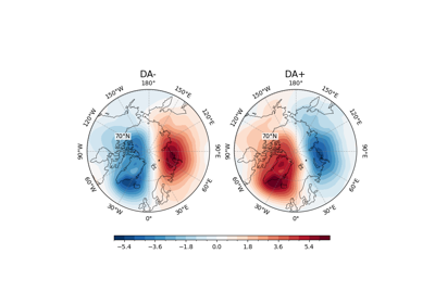
- easyclimate.field.teleconnection.calc_index_DA_EOF2_Wu_2006(slp_monthly_data: xarray.DataArray, time_range: slice = slice(None, None), lon_dim: str = 'lon', lat_dim: str = 'lat', lat_range: slice = slice(70, 90), time_dim: str = 'time', random_state: int | None = None, solver: Literal['auto', 'full', 'randomized'] = 'auto', solver_kwargs: dict = {}, normalized: bool = True) xarray.DataArray
The calculation of monthly mean Arctic Dipole Anomaly (DA/AD) index using empirical orthogonal functions (EOFs) method
Tip
The second EOF mode of SLP anomaly north of 70°N is Arctic Dipole Anomaly (DA/AD) pattern.
Parameters
- slp_monthly_data:
xarray.DataArray. The monthly data of sea level pressure (SLP).
- time_range:
slice, default: slice(None, None). The time range of seasonal cycle means to be calculated. The default value is the entire time range.
- lon_dim:
str, default: lon. Longitude coordinate dimension name. By default extracting is applied over the lon dimension.
- lat_dim:
str, default: lat. Latitude coordinate dimension name. By default extracting is applied over the lat dimension.
- lat_range:
slice, default: slice(20, 90). The latitude range of computation using EOFs over the Northern Hemisphere. The default value is from \(\mathrm{20^{\circ}N}\) to \(\mathrm{90^{\circ}N}\).
- time_dim:
str, default: time. The time coordinate dimension name.
- random_state:
int, default None. Seed for the random number generator.
- solver: {“auto”, “full”, “randomized”}, default: “auto”.
Solver to use for the EOFs computation.
- solver_kwargs:
dict, default {}. Additional keyword arguments to be passed to the EOFs solver.
- normalized:
bool, default True, optional. Whether to standardize the index based on standard deviation over time_range.
Returns
The monthly mean DA/AD index (
xarray.DataArray).Reference
Wu, B., Wang, J., & Walsh, J. E. (2006). Dipole Anomaly in the Winter Arctic Atmosphere and Its Association with Sea Ice Motion. Journal of Climate, 19(2), 210-225. https://doi.org/10.1175/JCLI3619.1
Wu, B., and M. A. Johnson (2007), A seesaw structure in SLP anomalies between the Beaufort Sea and the Barents Sea, Geophys. Res. Lett., 34, L05811, doi: https://doi.org/10.1029/2006GL028333.
Wang, J., J. Zhang, E. Watanabe, M. Ikeda, K. Mizobata, J. E. Walsh, X. Bai, and B. Wu (2009), Is the Dipole Anomaly a major driver to record lows in Arctic summer sea ice extent? Geophys. Res. Lett., 36, L05706, doi: https://doi.org/10.1029/2008GL036706.
Zhang, R. Zhang, Mechanisms for low-frequency variability of summer Arctic sea ice extent, Proc. Natl. Acad. Sci. U.S.A. 112 (15) 4570-4575, https://doi.org/10.1073/pnas.1422296112 (2015).
Kapsch, ML., Skific, N., Graversen, R.G. et al. Summers with low Arctic sea ice linked to persistence of spring atmospheric circulation patterns. Clim Dyn 52, 2497–2512 (2019). https://doi.org/10.1007/s00382-018-4279-z
Bi, H., Wang, Y., Liang, Y., Sun, W., Liang, X., Yu, Q., Zhang, Z., & Xu, X. (2021). Influences of Summertime Arctic Dipole Atmospheric Circulation on Sea Ice Concentration Variations in the Pacific Sector of the Arctic during Different Pacific Decadal Oscillation Phases. Journal of Climate, 34(8), 3003-3019. https://doi.org/10.1175/JCLI-D-19-0843.1
Bi, H., Liang, Y., & Chen, X. (2023). Distinct role of a spring atmospheric circulation mode in the Arctic sea ice decline in summer. Journal of Geophysical Research: Atmospheres, 128, e2022JD037477. https://doi.org/10.1029/2022JD037477
See also
Arctic Dipole Anomaly (DA/AD) and Barents-Beaufort Oscillation (BBO)
Arctic Dipole Anomaly (DA/AD) and Barents-Beaufort Oscillation (BBO)- slp_monthly_data: