easyclimate.core.eddy
The calculation of transient eddy
Functions
|
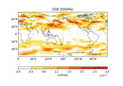
Calculate the maximum Eady growth rate. |
|
Calculate the apparent heat source. |
|
Calculate the total diabatic heating. |
|
Calculate the apparent moisture sink. |
|
Calculate Plumb wave activity horizontal flux. |
|
Calculate TN wave activity horizontal flux. |
|
Calculate horizontal Eliassen–Palm Flux. |
|
Calculate the Rossby wave source following Sardeshmukh and Hoskins (1988). |
Module Contents
- easyclimate.core.eddy.calc_eady_growth_rate(u_daily_data: xarray.DataArray, z_daily_data: xarray.DataArray, temper_daily_data: xarray.DataArray, vertical_dim: str, vertical_dim_units: Literal['hPa', 'Pa', 'mbar'], lat_dim: str = 'lat') xarray.Dataset
Calculate the maximum Eady growth rate.
\[\sigma = 0.3098 \frac{f}{N} \frac{\mathrm{d} U}{\mathrm{d} z}\]Caution
Eady growth rate (EGR) is a non-linear quantity. Hence, calc_eady_growth_rate should NOT be directly applied to monthly means variables. If a monthly climatology of EGR is desired, the EGR values at the high frequency temporal time steps should be calculated; then, use calculate monthly mean.
Parameters
- u_daily_data:
xarray.DataArray. The zonal wind daily data.
- z_daily_data:
xarray.DataArray. Daily atmospheric geopotential height.
Attention
The unit of z_daily_data should be meters, NOT \(\mathrm{m^2 \cdot s^2}\) which is the unit used in the representation of potential energy.
- temper_data:
xarray.DataArray. Daily air temperature.
- vertical_dim:
str. Vertical coordinate dimension name.
- vertical_dim_units:
str. The unit corresponding to the vertical p-coordinate value. Optional values are hPa, Pa, mbar.
- lat_dim:
str, default: lat. Latitude coordinate dimension name. By default extracting is applied over the lat dimension.
Returns
The maximum Eady growth rate (
xarray.Dataset).eady_growth_rate: The maximum Eady growth rate.
dudz: \(\frac{\mathrm{d} U}{\mathrm{d} z}\)
brunt_vaisala_frequency: Brunt-väisälä frequency.
See also
Eady, E. T. (1949). Long Waves and Cyclone Waves. Tellus, 1(3), 33–52. https://doi.org/10.3402/tellusa.v1i3.8507, https://www.tandfonline.com/doi/abs/10.3402/tellusa.v1i3.8507
Lindzen, R. S. , & Farrell, B. (1980). A Simple Approximate Result for the Maximum Growth Rate of Baroclinic Instabilities. Journal of Atmospheric Sciences, 37(7), 1648-1654. https://journals.ametsoc.org/view/journals/atsc/37/7/1520-0469_1980_037_1648_asarft_2_0_co_2.xml
Simmonds, I., and E.-P. Lim (2009), Biases in the calculation of Southern Hemisphere mean baroclinic eddy growth rate, Geophys. Res. Lett., 36, L01707, https://doi.org/10.1029/2008GL036320.
Sloyan, B. M., and T. J. O’Kane (2015), Drivers of decadal variability in the Tasman Sea, J. Geophys. Res. Oceans, 120, 3193–3210, https://doi.org/10.1002/2014JC010550.
- u_daily_data:
- easyclimate.core.eddy.calc_apparent_heat_source(u_data: xarray.DataArray, v_data: xarray.DataArray, omega_data: xarray.DataArray, temper_data: xarray.DataArray, vertical_dim: str, vertical_dim_units: Literal['hPa', 'Pa', 'mbar'], time_units: str, lon_dim='lon', lat_dim='lat', time_dim='time', c_p=1005.7) xarray.DataArray
Calculate the apparent heat source.
\[Q_1 = C_p \frac{T}{\theta} \left( \frac{\partial \theta}{\partial t} + u \frac{\partial \theta}{\partial x} + v \frac{\partial \theta}{\partial y} + \omega \frac{\partial \theta}{\partial p} \right)\]Parameters
- u_data:
xarray.DataArray. The zonal wind data.
- v_data:
xarray.DataArray. The meridional wind data.
- omega_data:
xarray.DataArray. The vertical velocity data (\(\frac{\mathrm{d} p}{\mathrm{d} t}\)).
- temper_data:
xarray.DataArray. Air temperature.
- vertical_dim:
str. Vertical coordinate dimension name.
- vertical_dim_units:
str. The unit corresponding to the vertical p-coordinate value. Optional values are hPa, Pa, mbar.
- time_units:
str. The unit corresponding to the time dimension value. Optional values are seconds, months, years and so on.
- lon_dim:
str, default: lon. Longitude coordinate dimension name. By default extracting is applied over the lon dimension.
- lat_dim:
str, default: lat. Latitude coordinate dimension name. By default extracting is applied over the lat dimension.
- time_dim:
str. The time coordinate dimension name.
- c_p:
float, default: 1005.7. The specific heat at constant pressure of dry air.
Returns
The apparent heat source (
xarray.DataArray).See also
- u_data:
- easyclimate.core.eddy.calc_total_diabatic_heating(u_data: xarray.DataArray, v_data: xarray.DataArray, omega_data: xarray.DataArray, temper_data: xarray.DataArray, vertical_dim: str, vertical_dim_units: Literal['hPa', 'Pa', 'mbar'], time_units: str, lat_dim='lat', lon_dim='lon', time_dim='time', c_p=1005.7) xarray.DataArray
Calculate the total diabatic heating.
Calculated in exactly the same way as for the apparent heat source.
Parameters
- u_data:
xarray.DataArray. The zonal wind data.
- v_data:
xarray.DataArray. The meridional wind data.
- omega_data:
xarray.DataArray. The vertical velocity data (\(\frac{\mathrm{d} p}{\mathrm{d} t}\)).
- temper_data:
xarray.DataArray. Air temperature.
- vertical_dim:
str. Vertical coordinate dimension name.
- vertical_dim_units:
str. The unit corresponding to the vertical p-coordinate value. Optional values are hPa, Pa, mbar.
- time_units:
str. The unit corresponding to the time dimension value. Optional values are seconds, months, years and so on.
- lon_dim:
str, default: lon. Longitude coordinate dimension name. By default extracting is applied over the lon dimension.
- lat_dim:
str, default: lat. Latitude coordinate dimension name. By default extracting is applied over the lat dimension.
- time_dim:
str, default: time. The time coordinate dimension name.
- c_p:
float, default: 1005.7 (\(\mathrm{J \cdot kg^{-1} \cdot K^{-1}}\)). The specific heat at constant pressure of dry air.
Returns
The total diabatic heating (
xarray.DataArray).See also
- u_data:
- easyclimate.core.eddy.calc_apparent_moisture_sink(u_data: xarray.DataArray, v_data: xarray.DataArray, omega_data: xarray.DataArray, specific_humidity_data: xarray.DataArray, vertical_dim: str, vertical_dim_units: Literal['hPa', 'Pa', 'mbar'], time_units: str, specific_humidity_data_units: str, lon_dim='lon', lat_dim='lat', time_dim='time', latent_heat_of_condensation=2501000.0) xarray.DataArray
Calculate the apparent moisture sink.
\[Q_2 = -L \left( \frac{\partial q}{\partial t} + u \frac{\partial q}{\partial x} + v \frac{\partial q}{\partial y} + \omega \frac{\partial q}{\partial p} \right)\]Parameters
- u_data:
xarray.DataArray. The zonal wind data.
- v_data:
xarray.DataArray. The meridional wind data.
- omega_data:
xarray.DataArray. The vertical velocity data (\(\frac{\mathrm{d} p}{\mathrm{d} t}\)).
- specific_humidity_data:
xarray.DataArray. The absolute humidity data.
- vertical_dim:
str. Vertical coordinate dimension name.
- vertical_dim_units:
str. The unit corresponding to the vertical p-coordinate value. Optional values are hPa, Pa, mbar.
- time_units:
str. The unit corresponding to the time dimension value. Optional values are seconds, months, years and so on.
- specific_humidity_data_units:
str. The unit corresponding to specific_humidity value. Optional values are kg/kg, g/kg and so on.
- lon_dim:
str, default: lon. Longitude coordinate dimension name. By default extracting is applied over the lon dimension.
- lat_dim:
str, default: lat. Latitude coordinate dimension name. By default extracting is applied over the lat dimension.
- time_dim:
str, default: time. The time coordinate dimension name.
- latent_heat_of_condensation:
float, default: 2.5008e6 (\(\mathrm{J \cdot kg^{-1}}\)). Latent heat of condensation of water at 0°C.
Returns
The apparent moisture sink (
xarray.DataArray).See also
- u_data:
- easyclimate.core.eddy.calc_Plumb_wave_activity_horizontal_flux(z_prime_data: xarray.DataArray, vertical_dim: str, vertical_dim_units: Literal['hPa', 'Pa', 'mbar'], lon_dim='lon', lat_dim='lat', omega=7.292e-05, g=9.8, R=6370000) xarray.Dataset
Calculate Plumb wave activity horizontal flux.
Parameters
- z_prime_data:
xarray.DataArray. The anormaly of atmospheric geopotential height.
- vertical_dim:
str. Vertical coordinate dimension name.
- vertical_dim_units:
str. The unit corresponding to the vertical p-coordinate value. Optional values are hPa, Pa, mbar.
- lon_dim:
str, default: lon. Longitude coordinate dimension name. By default extracting is applied over the lon dimension.
- lat_dim:
str, default: lat. Latitude coordinate dimension name. By default extracting is applied over the lat dimension.
- omega:
float, default: 7.292e-5. The angular speed of the earth.
- g:
float, default: 9.8. The acceleration of gravity.
- R:
float, default: 6370000. Radius of the Earth.
Returns
The Plumb wave activity horizontal flux (
xarray.DataArray).- z_prime_data:
- easyclimate.core.eddy.calc_TN_wave_activity_horizontal_flux(z_prime_data: xarray.DataArray | None, u_climatology_data: xarray.DataArray, v_climatology_data: xarray.DataArray, vertical_dim: str, vertical_dim_units: Literal['hPa', 'Pa', 'mbar'], psi_prime_data: xarray.DataArray | None = None, lon_dim: str = 'lon', lat_dim: str = 'lat', time_dim: str = 'time', omega: float = 7.292e-05, g: float = 9.8, R: float = 6371200.0) xarray.Dataset
Calculate TN wave activity horizontal flux.
\[\begin{split}\mathbf{W_h} = \frac{p\cos\varphi}{2\lvert \mathbf{U_c} \rvert}\begin{pmatrix} \frac{U_c}{R^2 \cos^2 \varphi} \left[ \left( \frac{\partial \psi'}{\partial \lambda} \right)^2 - \psi'\frac{\partial^2 \psi'}{\partial \lambda^2} \right] + \frac{V_c}{R^2 \cos \varphi} \left[ \frac{\partial \psi'}{\partial \lambda} \frac{\partial \psi'}{\partial \varphi} - \psi' \frac{\partial^2 \psi'}{\partial \lambda \partial \varphi} \right] \\ \frac{U_c}{R^2 \cos \varphi} \left[ \frac{\partial \psi'}{\partial \lambda} \frac{\partial \psi'}{\partial \varphi} - \psi' \frac{\partial^2 \psi'}{\partial \lambda \partial \varphi} \right] + \frac{V_c}{R^2} \left[ \left( \frac{\partial \psi'}{\partial \varphi} \right)^2 - \psi'\frac{\partial^2 \psi'}{\partial \varphi^2} \right] \\ \end{pmatrix}\end{split}\]Parameters
- z_prime_data:
xarray.DataArray. The anormaly of atmospheric geopotential height.
Attention
The unit of z_prime_data should be meters, NOT \(\mathrm{m^2 \cdot s^2}\) which is the unit used in the representation of potential energy.
- u_climatology_data:
xarray.DataArray. The climatology of zonal wind data.
- v_climatology_data:
xarray.DataArray. The climatology of meridional wind data.
- vertical_dim:
str. Vertical coordinate dimension name.
- vertical_dim_units:
str. The unit corresponding to the vertical p-coordinate value. Optional values are hPa, Pa, mbar.
- psi_prime_data:
xarray.DataArray. Perturbation stream function. Geostrophic stream function perturbation calculated from geopotential height anomaly.
- lon_dim:
str, default: lon. Longitude coordinate dimension name. By default extracting is applied over the lon dimension.
- lat_dim:
str, default: lat. Latitude coordinate dimension name. By default extracting is applied over the lat dimension.
- omega:
float, default: 7.292e-5. The angular speed of the earth.
- g:
float, default: 9.8. The acceleration of gravity.
- R:
float, default: 6370000. Radius of the Earth.
Returns
The TN wave activity horizontal flux (
xarray.Dataset).Reference
Takaya, K., & Nakamura, H. (2001). A Formulation of a Phase-Independent Wave-Activity Flux for Stationary and Migratory Quasigeostrophic Eddies on a Zonally Varying Basic Flow. Journal of the Atmospheric Sciences, 58(6), 608-627. https://journals.ametsoc.org/view/journals/atsc/58/6/1520-0469_2001_058_0608_afoapi_2.0.co_2.xml
- z_prime_data:
- easyclimate.core.eddy.calc_EP_horizontal_flux(u_prime_data: xarray.DataArray, v_prime_data: xarray.DataArray, time_dim: str = 'time', lat_dim: str = 'lat') xarray.Dataset
Calculate horizontal Eliassen–Palm Flux.
Parameters
- u_prime_data:
xarray.DataArray. The anormaly of zonal wind data.
- v_prime_data:
xarray.DataArray. The anormaly of meridional wind data.
- time_dim:
str, default: time. The time coordinate dimension name.
- lat_dim:
str, default: lat. Latitude coordinate dimension name. By default extracting is applied over the lat dimension.
Returns
The Eliassen–Palm Flux (
xarray.DataArray).- u_prime_data:
- easyclimate.core.eddy.calc_monthly_rossby_wave_source(u_data: xarray.DataArray, v_data: xarray.DataArray, u_climatology_data: xarray.DataArray, v_climatology_data: xarray.DataArray, lat_dim: str = 'lat', omega: float = 7.292e-05, R: float = 6371200.0) xarray.DataArray
Calculate the Rossby wave source following Sardeshmukh and Hoskins (1988).
The Rossby wave source (RWS) represents the forcing term for stationary Rossby waves and is widely used to diagnose atmospheric teleconnections. It is decomposed into five terms representing different physical mechanisms:
\[S' = -\nabla \cdot (\mathbf{v}_\chi \zeta)' = \text{term1a} + \text{term1b} + \text{term2a} + \text{term2b} + \text{term3} + \text{term4} + \text{term5}\]where:
term1a: \(-\bar{\zeta} \nabla \cdot \mathbf{v}'_\chi\) (stretching of climatological vorticity by divergent wind anomalies)
Term1b: \(-f \nabla \cdot \mathbf{v'_\chi}\) (Stretching of planetary vorticity by anomalous divergence)
term2a: \(-\mathbf{v}'_\chi \cdot \nabla\bar{\zeta}\) (advection of climatological vorticity by divergent wind anomalies)
term2b: \(-\beta v'_\chi\) (planetary vorticity advection, where \(\beta = \partial f/\partial y\))
term3: \(-\zeta' \nabla \cdot \bar{\mathbf{v}}_\chi\) (stretching of vorticity anomalies by climatological divergent wind)
term4: \(-\bar{\mathbf{v}}_\chi \cdot \nabla\zeta'\) (advection of vorticity anomalies by climatological divergent wind)
term5: \(-\nabla \cdot (\mathbf{v}'_\chi \zeta')\) (nonlinear term: divergence of transient vorticity flux)
where \(\mathbf{v}_\chi = (u_\chi, v_\chi)\) is the divergent (irrotational) wind component, \(\zeta\) is relative vorticity, overbar denotes climatology, and prime denotes anomaly.
Note
Anomalies are computed as deviations from the monthly climatology.
The planetary term (term6) represents the beta effect, which is important for Rossby wave propagation, especially in the tropics and subtropics.
Terms 1, 2, and 6 typically dominate the Rossby wave source.
Positive RWS indicates a cyclonic wave source; negative indicates anticyclonic.
Parameters
- u_data
xarray.DataArray(\(\mathrm{m/s}\)) Zonal wind component. Must contain a ‘time’ dimension with monthly or higher frequency data. Expected dimensions:
(time, lat, lon)or(time, level, lat, lon).- v_data
xarray.DataArray(\(\mathrm{m/s}\)) Meridional wind component. Must have the same dimensions as u_data.
- u_climatology_data
xarray.DataArray(\(\mathrm{m/s}\)) Monthly climatology of zonal wind. Expected dimensions:
(time, lat, lon)or(time, level, lat, lon), where time/month ranges from 1 to 12.- v_climatology_data
xarray.DataArray(\(\mathrm{m/s}\)) Monthly climatology of meridional wind. Must have the same dimensions as u_climatology_data.
Returns
- result
xarray.Dataset Dataset containing the Rossby wave source and its five decomposed terms:
RWS: Total Rossby wave source (sum of all terms)
term1a: Vorticity stretching by anomalous divergence
term1b: Stretching of planetary vorticity by anomalous divergence
term2a: Vorticity advection by anomalous divergent wind
term2b: Planetary vorticity advection (beta effect)
term3: Anomalous vorticity stretching by climatological divergence
term4: Anomalous vorticity advection by climatological divergent wind
term5: Nonlinear transient eddy term
All variables have units of \(\mathrm{s^{-2}}\) and retain the spatial/temporal dimensions of the input data.
See also
Sardeshmukh, P. D., & Hoskins, B. J. (1988). The generation of global rotational flow by steady idealized tropical divergence. Journal of the Atmospheric Sciences, 45(7), 1228-1251. https://journals.ametsoc.org/view/journals/atsc/45/7/1520-0469_1988_045_1228_tgogrf_2_0_co_2.xml, https://doi.org/10.1175/1520-0469(1988)045<1228:TGOGRF>2.0.CO;2
Examples
>>> # Calculate monthly climatology
>>> u_clim = u.groupby('time.month').mean('time')
>>> v_clim = v.groupby('time.month').mean('time')
>>>
>>> # Compute Rossby wave source
>>> rws_result = calc_rossby_wave_source(u, v, u_clim, v_clim)
>>>
>>> # Visualize the dominant terms
>>> rws_result['RWS'].sel(time='2015-12').plot()
>>> (rws_result['term1'] + rws_result['term2']).sel(time='2015-12').plot()