easyclimate.core.spec.plot¶

Visualization for spherical harmonics analysis

Functions¶

`spectral_coefficients_to_matrix`(→ xarray.DataArray)	Convert packed triangular spectral coefficients to an `(m, n)` matrix.
`spectral_power_by_total_wavenumber`(→ xarray.DataArray)	Sum spectral power over zonal wavenumber for each total wavenumber.
`plot_spectral_power`(spec[, ax, logy, grid])	Plot spectral power as a function of total wavenumber.
`plot_spectral_matrix`(spec[, value, ax, cmap, add_colorbar])	Plot a packed triangular spectral coefficient field as an m-n matrix.
`plot_spectral_real_imag`(spec[, figsize, cmap])	Plot real and imaginary parts of packed triangular spectral coefficients.

Module Contents¶

easyclimate.core.spec.plot.spectral_coefficients_to_matrix(spec: xarray.DataArray, value: str = 'abs', eps: float = 1e-30, mode: str = 'spec_dim') → xarray.DataArray¶

Convert packed triangular spectral coefficients to an (m, n) matrix.

The input coefficients are assumed to follow triangular spherical-harmonic ordering, where the packed dimension contains all pairs with 0 <= m <= n <= ntrunc. Cells outside the triangular domain (n < m) are filled with NaN in the returned matrix.

Parameters¶

specxr.DataArray: One-dimensional spectral coefficients. Select non-mode dimensions first, e.g. spec_data.isel(time=0, level=0).
value{“abs”, “logabs”, “power”, “real”, “imag”}: Which quantity to place in the matrix.
epsfloat: Small number used only for logabs.
modestr, default: “spec_dim”: Name of the packed spectral coefficient dimension.

Returns¶

xr.DataArray: Two-dimensional coefficient matrix with dimensions ("m", "n").

Visualization for Spherical Harmonics

easyclimate.core.spec.plot.spectral_power_by_total_wavenumber(spec: xarray.DataArray, mode: str = 'spec_dim') → xarray.DataArray¶

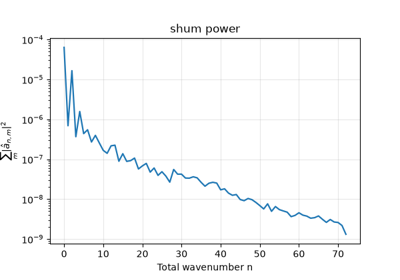
Sum spectral power over zonal wavenumber for each total wavenumber.

The returned one-dimensional spectrum is \(E(n) = \sum_m |\hat{a}_{n,m}|^2\) for packed triangular spherical-harmonic coefficients.

Parameters¶

specxr.DataArray: One-dimensional spectral coefficients. Select non-mode dimensions first, e.g. spec_data.isel(time=0, level=0).
modestr, default: “spec_dim”: Name of the packed spectral coefficient dimension.

Returns¶

xr.DataArray: Spectral power indexed by total wavenumber n.

Visualization for Spherical Harmonics

easyclimate.core.spec.plot.plot_spectral_power(spec: xarray.DataArray, ax=None, logy: bool = True, grid: bool = True, **plot_kwargs)¶

Plot spectral power as a function of total wavenumber.

This function first sums the packed triangular spectral coefficients over zonal wavenumber m with spectral_power_by_total_wavenumber(), then draws \(E(n) = \sum_m |\hat{a}_{n,m}|^2\) against total wavenumber n.

Parameters¶

specxr.DataArray: One-dimensional packed triangular spectral coefficients. If the input data has time, level, or other non-spectral dimensions, select one slice before plotting, e.g. spec.isel(time=0).
axmatplotlib.axes.Axes, optional: Axes used for drawing. If None, a new figure and axes are created.
logybool, default: True: If True, draw the spectrum with a logarithmic y-axis by calling matplotlib.axes.Axes.semilogy(). If False, call matplotlib.axes.Axes.plot().
gridbool, default: True: Whether to add a light grid to the axes.
**plot_kwargs: Additional keyword arguments passed to ax.semilogy or ax.plot.

Returns¶

tuple: (fig, ax), where fig is the Matplotlib figure and ax is the axes containing the spectrum.

Visualization for Spherical Harmonics

easyclimate.core.spec.plot.plot_spectral_matrix(spec: xarray.DataArray, value: str = 'logabs', ax=None, cmap: str = 'viridis', add_colorbar: bool = True, **imshow_kwargs)¶

Plot a packed triangular spectral coefficient field as an m-n matrix.

The packed spectral dimension is reshaped to a triangular matrix whose rows are zonal wavenumber m and columns are total wavenumber n. Matrix cells with n < m are outside the triangular spectral domain and are shown as NaN.

Parameters¶

specxr.DataArray

One-dimensional packed triangular spectral coefficients. Select any non-spectral dimensions before plotting.

value{“abs”, “logabs”, “power”, “real”, “imag”}, default: “logabs”

Quantity to visualize:

"abs": coefficient magnitude.
"logabs": base-10 logarithm of coefficient magnitude.
"power": squared coefficient magnitude.
"real": real part of the coefficient.
"imag": imaginary part of the coefficient.

axmatplotlib.axes.Axes, optional

Axes used for drawing. If None, a new axes is created.

cmapstr, default: “viridis”

Matplotlib colormap used by matplotlib.axes.Axes.imshow().

add_colorbarbool, default: True

Whether to add a colorbar for the plotted matrix.

**imshow_kwargs

Additional keyword arguments passed to ax.imshow. The defaults are origin="lower" and aspect="auto" unless explicitly provided.

Returns¶

matplotlib.axes.Axes: Axes containing the coefficient matrix image.

Visualization for Spherical Harmonics

easyclimate.core.spec.plot.plot_spectral_real_imag(spec: xarray.DataArray, figsize: tuple[float, float] = (11, 4), cmap: str = 'viridis', **imshow_kwargs)¶

Plot real and imaginary parts of packed triangular spectral coefficients.

This is a convenience wrapper around plot_spectral_matrix(). It creates a two-panel figure and draws value="real" in the left panel and value="imag" in the right panel.

Parameters¶

specxr.DataArray: One-dimensional packed triangular spectral coefficients. Select any non-spectral dimensions before plotting.
figsizetuple of float, default: (11, 4): Matplotlib figure size passed to matplotlib.pyplot.subplots().
cmapstr, default: “viridis”: Matplotlib colormap used for both matrix panels.
**imshow_kwargs: Additional keyword arguments passed to plot_spectral_matrix() and then to ax.imshow for both panels.

Returns¶

tuple: (fig, ax), where fig is the Matplotlib figure and ax is the two-element array of axes containing the real and imaginary matrices.

Visualization for Spherical Harmonics