
Note
Go to the end to download the full example code.
Tools for Spherical Harmonics
This page introduces low-level helpers for spherical-harmonic grids and
triangular spectral indexing. Each function is available in both the standard
backend and a Rust-backed *_rs variant where applicable.
import easyclimate as ecl
import numpy as np
import matplotlib.pyplot as plt
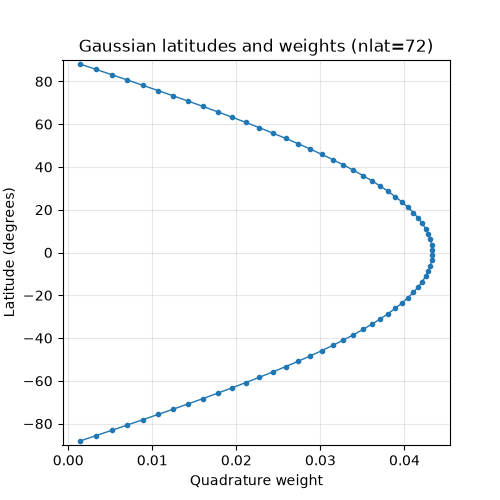
Gaussian latitudes are the latitude nodes used by spherical-harmonic transforms on Gaussian grids. The quadrature weights indicate how much each latitude contributes to the Gaussian integration over the sphere.
The weights are largest near the equator and decrease toward the poles, reflecting the spherical area represented by each latitude band. The latitude nodes and weights are symmetric about the equator.
ecl.spec.calc_gaussian_latitudes(72)
ecl.spec.calc_gaussian_latitudes_rs(72)
The returned dataset contains both the Gaussian latitude nodes and their quadrature weights. To show how the Gaussian grid is distributed in latitude, we plot the quadrature weight as a function of latitude.
The result should be symmetric about the equator. The weights are largest near the equator and decrease toward the poles, reflecting the smaller effective area represented by high-latitude bands.
nlat = 72
gauss = ecl.spec.calc_gaussian_latitudes(nlat)

lats = gauss["lats"].values
wts = gauss["wts"].values

fig, ax = plt.subplots(figsize=(5, 5))
ax.plot(wts, lats, marker="o", markersize=3, linewidth=1)

ax.set_title(f"Gaussian latitudes and weights (nlat={nlat})")
ax.set_xlabel("Quadrature weight")
ax.set_ylabel("Latitude (degrees)")
ax.set_ylim(-90, 90)
ax.grid(alpha=0.3)
%%
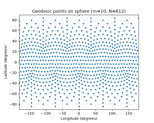
Geodesic points are nearly evenly distributed points on the sphere generated
from an icosahedral geodesic. The parameter m controls the number of
points along one edge of a geodesic triangle.
For m = 10, the total number of points is 10 * (m - 1)**2 + 2 = 812.
Here the points are plotted in longitude-latitude coordinates. The apparent
deformation at high latitudes comes from the longitude-latitude projection,
rather than from nonuniformity on the sphere.
ecl.spec.calc_geodesic_points(10)
ecl.spec.calc_geodesic_points_rs(10)
The geodesic helper returns point locations on the sphere as longitude and latitude arrays. Here we plot these points in a simple longitude-latitude coordinate system.
The points are nearly evenly distributed on the sphere, but the lon-lat view is not an equal-area projection. Therefore, apparent compression or waviness at high latitudes mainly reflects the map projection rather than an error in the geodesic construction.
m_geo = 10
geo = ecl.spec.calc_geodesic_points(m_geo)

lons = geo["lons"].values
lats = geo["lats"].values
lons = ((lons + 180) % 360) - 180

fig, ax = plt.subplots(figsize=(6, 4.8))
ax.scatter(lons, lats, s=10)

ax.set_title(f"Geodesic points on sphere (m={m_geo}, N={lats.size})")
ax.set_xlabel("Longitude (degrees)")
ax.set_ylabel("Latitude (degrees)")
ax.set_xlim(-180, 180)
ax.set_ylim(-90, 90)
ax.grid(alpha=0.3)
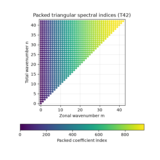
Spherical-harmonic coefficients are stored in a packed triangular order.
For triangular truncation Tntrunc, only coefficient pairs satisfying
0 <= m <= n <= ntrunc are retained.
This plot maps the one-dimensional packed coefficient index back to the
two-dimensional spectral-index space (m, n). It is useful for interpreting
spectral coefficients returned by spherical-harmonic transforms.
ecl.spec.calc_spherical_harmonic_coefficients(42)
ecl.spec.calc_spherical_harmonic_coefficients_rs(42)
The spectral coefficients are stored in a one-dimensional packed array, but
each coefficient corresponds to a pair of spherical-harmonic indices:
zonal wavenumber m and total wavenumber n.
This plot maps the packed coefficient index back to the triangular (m, n)
layout. For triangular truncation T42, only coefficients satisfying
0 <= m <= n <= 42 are retained.
ntrunc = 42
coef = ecl.spec.calc_spherical_harmonic_coefficients(ntrunc)

indxm = coef["indxm"].values
indxn = coef["indxn"].values
packed_index = np.arange(indxm.size)

fig, ax = plt.subplots(figsize=(5.5, 5.5))
sc = ax.scatter(indxm, indxn, c=packed_index, s=14)

ax.set_title(f"Packed triangular spectral indices (T{ntrunc})")
ax.set_xlabel("Zonal wavenumber m")
ax.set_ylabel("Total wavenumber n")
ax.set_xlim(-1, ntrunc + 1)
ax.set_ylim(-1, ntrunc + 1)
ax.set_aspect("equal", adjustable="box")
ax.grid(alpha=0.3)

cbar = fig.colorbar(sc, ax=ax, orientation = 'horizontal')
cbar.set_label("Packed coefficient index")
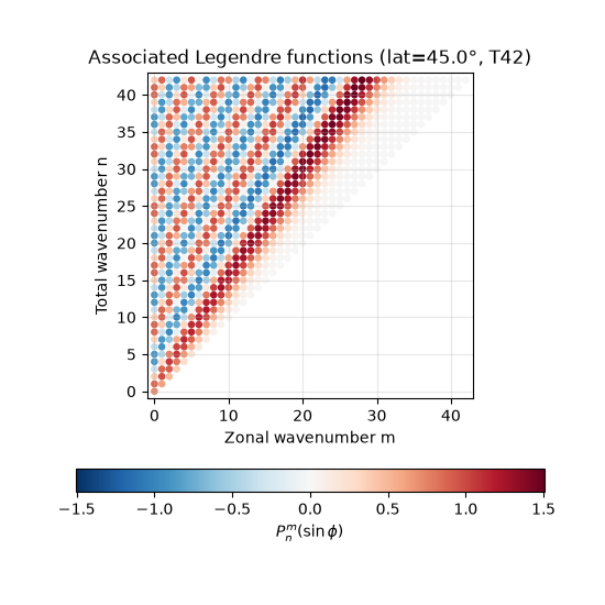
Associated Legendre functions are the latitude-dependent part of the spherical-harmonic basis. For a given latitude and triangular truncation, the function returns one value for each packed spectral coefficient.
Here the one-dimensional output is displayed on the same triangular
(m, n) layout used by the spherical-harmonic coefficient indices.
Positive and negative values are shown with a diverging color map.
ecl.spec.calc_legendre_functions(45.0, 42)
ecl.spec.calc_legendre_functions_rs(45.0, 42)
The associated Legendre functions form the latitude-dependent part of the spherical-harmonic basis. For a fixed latitude and triangular truncation, the returned values follow the same packed triangular order as the spectral coefficients.
We therefore reuse calc_spherical_harmonic_coefficients to recover the
corresponding (m, n) coordinates, and then display the Legendre-function
values on this triangular spectral layout.
lat0 = 45.0
coef = ecl.spec.calc_spherical_harmonic_coefficients(42)
pnm = ecl.spec.calc_legendre_functions(lat0, 42)

indxm = coef["indxm"].values
indxn = coef["indxn"].values
pnm_values = np.asarray(pnm.values)

vmax = np.nanmax(np.abs(pnm_values))

fig, ax = plt.subplots(figsize=(5.5, 5.5))
sc = ax.scatter(
    indxm,
    indxn,
    c=pnm_values,
    s=14,
    cmap="RdBu_r",
    vmin=-vmax,
    vmax=vmax,
)

ax.set_title(f"Associated Legendre functions (lat={lat0}°, T42)")
ax.set_xlabel("Zonal wavenumber m")
ax.set_ylabel("Total wavenumber n")
ax.set_xlim(-1, 43)
ax.set_ylim(-1, 43)
ax.set_aspect("equal", adjustable="box")
ax.grid(alpha=0.3)

cbar = fig.colorbar(sc, ax=ax, orientation = 'horizontal')
cbar.set_label(r"$P_n^m(\sin \phi)$")
Total running time of the script: (0 minutes 4.183 seconds)