
Visualization for Spherical Harmonics

This example transforms a gridded field to packed triangular spectral coefficients, visualizes the spectral coefficients, and transforms the field back to latitude-longitude space. The standard backend and Rust-backed functions are compared with the same input data.

import numpy as np
import matplotlib.pyplot as plt
import easyclimate as ecl

Open a tutorial specific-humidity field. The spectral transform expects latitude and longitude dimensions on a regular or Gaussian global grid.

<xarray.DataArray 'shum' (time: 5, level: 8, lat: 73, lon: 144)> Size: 2MB
[420480 values with dtype=float32]
Coordinates:
  * time     (time) datetime64[ns] 40B 2022-01-01 2022-01-02 ... 2022-01-05
  * level    (level) float32 32B 1e+03 925.0 850.0 700.0 600.0 500.0 400.0 300.0
  * lat      (lat) float32 292B 90.0 87.5 85.0 82.5 ... -82.5 -85.0 -87.5 -90.0
  * lon      (lon) float32 576B 0.0 2.5 5.0 7.5 10.0 ... 350.0 352.5 355.0 357.5
Attributes:
    long_name:     mean Daily specific humidity
    units:         kg/kg
    precision:     6
    GRIB_id:       51
    GRIB_name:     SPFH
    var_desc:      Specific humidity
    level_desc:    Pressure Levels
    statistic:     Mean
    parent_stat:   Individual Obs
    dataset:       NCEP Reanalysis Daily Averages
    actual_range:  [0.        0.0463525]


Transform grid-space data to packed triangular spherical-harmonic coefficients. The output has a spec_dim dimension whose length is determined by the triangular truncation.

q_spec_data = ecl.spec.transfer_grid2spectral_transform(
    q_grid_data,
    grid_data_type = "regular"
)
q_spec_rs_data = ecl.spec.transfer_grid2spectral_transform_rs(
    q_grid_data,
    grid_data_type = "regular"
)
q_spec_data
<xarray.DataArray 'shum' (time: 5, level: 8, spec_dim: 2701)> Size: 864kB
array([[[ 1.4318056e-02+0.0000000e+00j, -1.6885565e-03+0.0000000e+00j,
         -7.4368455e-03+0.0000000e+00j, ...,
         -1.2462871e-06-7.9038989e-07j,  0.0000000e+00+0.0000000e+00j,
         -2.2851473e-06+0.0000000e+00j],
        [ 1.1034398e-02+0.0000000e+00j, -1.2108366e-03+0.0000000e+00j,
         -5.6361794e-03+0.0000000e+00j, ...,
         -2.6656276e-06-2.3535777e-06j,  0.0000000e+00+0.0000000e+00j,
         -5.3515367e-07+0.0000000e+00j],
        [ 7.9695480e-03+0.0000000e+00j, -8.1353396e-04+0.0000000e+00j,
         -4.0646000e-03+0.0000000e+00j, ...,
         -3.4380923e-06-2.0546772e-06j,  0.0000000e+00+0.0000000e+00j,
         -2.7374588e-06+0.0000000e+00j],
        ...,
        [ 1.5948373e-03+0.0000000e+00j, -2.0274927e-04+0.0000000e+00j,
         -7.3477556e-04+0.0000000e+00j, ...,
          5.8628126e-07+3.9806199e-07j,  0.0000000e+00+0.0000000e+00j,
         -3.2343485e-07+0.0000000e+00j],
        [ 8.6961855e-04+0.0000000e+00j, -1.1698594e-04+0.0000000e+00j,
         -4.4932778e-04+0.0000000e+00j, ...,
          3.1276281e-07-7.4020505e-08j,  0.0000000e+00+0.0000000e+00j,
...
         -1.4971976e-06-4.9508976e-06j,  0.0000000e+00+0.0000000e+00j,
         -1.2484895e-07+0.0000000e+00j],
        [ 7.9506906e-03+0.0000000e+00j, -9.1070065e-04+0.0000000e+00j,
         -4.0739458e-03+0.0000000e+00j, ...,
         -1.7599943e-06-3.1492236e-06j,  0.0000000e+00+0.0000000e+00j,
         -9.9916679e-07+0.0000000e+00j],
        ...,
        [ 1.6448544e-03+0.0000000e+00j, -2.1513145e-04+0.0000000e+00j,
         -7.2625553e-04+0.0000000e+00j, ...,
          3.9967392e-07-7.7032672e-07j,  0.0000000e+00+0.0000000e+00j,
          3.5275087e-07+0.0000000e+00j],
        [ 8.8744168e-04+0.0000000e+00j, -1.2000850e-04+0.0000000e+00j,
         -4.5085562e-04+0.0000000e+00j, ...,
          1.7273464e-07+3.6746229e-08j,  0.0000000e+00+0.0000000e+00j,
         -1.9313656e-07+0.0000000e+00j],
        [ 3.7447075e-04+0.0000000e+00j, -5.9238486e-05+0.0000000e+00j,
         -2.2076482e-04+0.0000000e+00j, ...,
         -7.8376395e-08+5.9142192e-08j,  0.0000000e+00+0.0000000e+00j,
         -9.2633741e-08+0.0000000e+00j]]],
      shape=(5, 8, 2701), dtype=complex64)
Coordinates:
  * time      (time) datetime64[ns] 40B 2022-01-01 2022-01-02 ... 2022-01-05
  * level     (level) float32 32B 1e+03 925.0 850.0 700.0 ... 500.0 400.0 300.0
  * spec_dim  (spec_dim) int64 22kB 0 1 2 3 4 5 ... 2696 2697 2698 2699 2700
Attributes: (12/14)
    long_name:     mean Daily specific humidity
    units:         kg/kg
    precision:     6
    GRIB_id:       51
    GRIB_name:     SPFH
    var_desc:      Specific humidity
    ...            ...
    parent_stat:   Individual Obs
    dataset:       NCEP Reanalysis Daily Averages
    actual_range:  [0.        0.0463525]
    Description:   Spherical harmonic coefficients
    Truncation:    Triangular truncation at wavenumber 72
    Order:         Complex coefficients in triangular order


The plotting helpers expect a one-dimensional spectral coefficient array, so select one time and level before visualizing the spectrum.

<xarray.DataArray 'shum' (spec_dim: 2701)> Size: 22kB
array([ 7.9695480e-03+0.0000000e+00j, -8.1353396e-04+0.0000000e+00j,
       -4.0646000e-03+0.0000000e+00j, ..., -3.4380923e-06-2.0546772e-06j,
        0.0000000e+00+0.0000000e+00j, -2.7374588e-06+0.0000000e+00j],
      shape=(2701,), dtype=complex64)
Coordinates:
  * spec_dim  (spec_dim) int64 22kB 0 1 2 3 4 5 ... 2696 2697 2698 2699 2700
    time      datetime64[ns] 8B 2022-01-01
    level     float32 4B 850.0
Attributes: (12/14)
    long_name:     mean Daily specific humidity
    units:         kg/kg
    precision:     6
    GRIB_id:       51
    GRIB_name:     SPFH
    var_desc:      Specific humidity
    ...            ...
    parent_stat:   Individual Obs
    dataset:       NCEP Reanalysis Daily Averages
    actual_range:  [0.        0.0463525]
    Description:   Spherical harmonic coefficients
    Truncation:    Triangular truncation at wavenumber 72
    Order:         Complex coefficients in triangular order


Plot the total-wavenumber power spectrum, computed as the sum of squared coefficient magnitude over zonal wavenumber.

ecl.spec.plot_spectral_power(q_spec_data_sample)
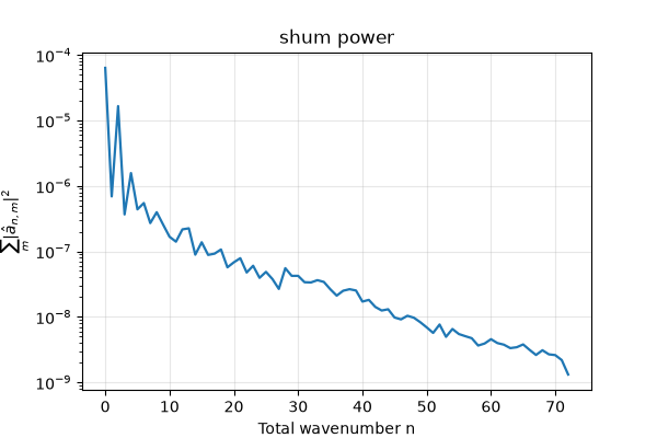
shum power
(<Figure size 600x400 with 1 Axes>, <Axes: title={'center': 'shum power'}, xlabel='Total wavenumber n', ylabel='$\\sum_m |\\hat{a}_{n,m}|^2$'>)

Plot the packed coefficients as an m by n triangular matrix. By default this displays the base-10 logarithm of coefficient magnitude.

ecl.spec.plot_spectral_matrix(q_spec_data_sample)
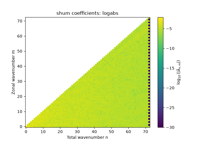
shum coefficients: logabs
<Axes: title={'center': 'shum coefficients: logabs'}, xlabel='Total wavenumber n', ylabel='Zonal wavenumber m'>

Plot the real and imaginary parts of the complex spectral coefficients in two side-by-side panels.

ecl.spec.plot_spectral_real_imag(q_spec_data_sample)
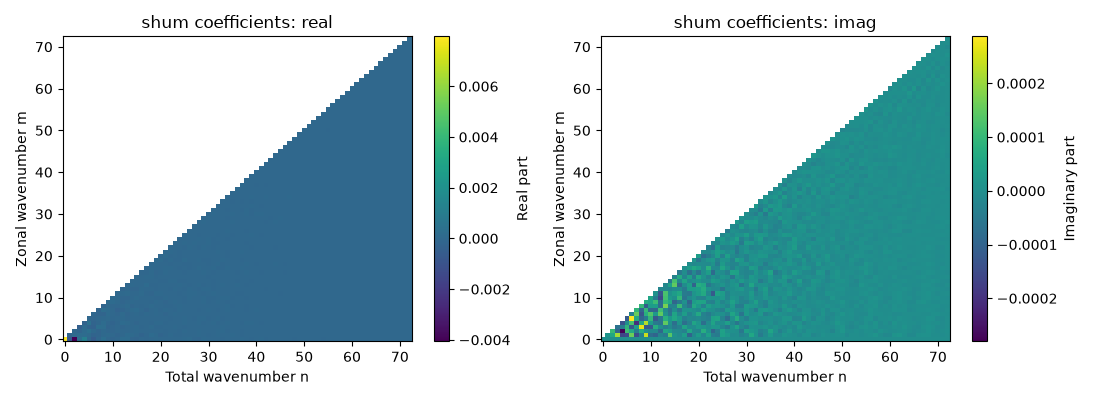
shum coefficients: real, shum coefficients: imag
(<Figure size 1100x400 with 4 Axes>, array([<Axes: title={'center': 'shum coefficients: real'}, xlabel='Total wavenumber n', ylabel='Zonal wavenumber m'>,
       <Axes: title={'center': 'shum coefficients: imag'}, xlabel='Total wavenumber n', ylabel='Zonal wavenumber m'>],
      dtype=object))

Transform the spectral coefficients back to grid space. The output grid size and grid type are supplied explicitly, matching the original regular grid.

q_grid_spectrans = ecl.spec.transfer_spectral_transform2grid(
    q_spec_data,
    nlon = 144, nlat = 73,
    grid_data_type = "regular"
)
q_grid_rs_spectrans = ecl.spec.transfer_spectral_transform2grid_rs(
    q_spec_rs_data,
    nlon = 144, nlat = 73,
    grid_data_type = "regular"
)
q_grid_spectrans
<xarray.DataArray 'shum' (time: 5, level: 8, lat: 73, lon: 144)> Size: 2MB
array([[[[ 3.75000411e-04,  3.75000178e-04,  3.75000178e-04, ...,
           3.75000294e-04,  3.75000411e-04,  3.75000178e-04],
         [ 1.54077774e-04,  1.49947475e-04,  1.46463630e-04, ...,
           1.70216314e-04,  1.64230005e-04,  1.58843468e-04],
         [ 2.86630588e-04,  3.15811252e-04,  3.41447070e-04, ...,
           1.95691711e-04,  2.24730000e-04,  2.55651423e-04],
         ...,
         [ 2.83718738e-03,  2.96073454e-03,  3.07869678e-03, ...,
           2.48415163e-03,  2.59390334e-03,  2.71319784e-03],
         [ 2.84030405e-03,  2.85255676e-03,  2.86575407e-03, ...,
           2.81346962e-03,  2.82037631e-03,  2.82944040e-03],
         [ 2.44500209e-03,  2.44500209e-03,  2.44500209e-03, ...,
           2.44500185e-03,  2.44500209e-03,  2.44500209e-03]],

        [[ 6.92499452e-04,  6.92499161e-04,  6.92499278e-04, ...,
           6.92499394e-04,  6.92499569e-04,  6.92499569e-04],
         [ 6.55071926e-04,  6.54639502e-04,  6.53355150e-04, ...,
           6.51236449e-04,  6.53356605e-04,  6.54642005e-04],
         [ 9.31355811e-04,  9.56825214e-04,  9.75400733e-04, ...,
           8.25620955e-04,  8.64318805e-04,  9.00070590e-04],
...
           4.24807076e-05,  4.16824041e-05,  4.25296566e-05],
         [ 2.81357097e-05,  2.90353328e-05,  3.01473665e-05, ...,
           2.67630821e-05,  2.70008932e-05,  2.74568556e-05],
         [ 4.74998888e-06,  4.74995977e-06,  4.74994886e-06, ...,
           4.75002162e-06,  4.75000343e-06,  4.75000343e-06]],

        [[ 3.02499830e-05,  3.02499811e-05,  3.02499793e-05, ...,
           3.02500175e-05,  3.02500048e-05,  3.02499902e-05],
         [ 2.97071783e-05,  2.89855743e-05,  2.82412384e-05, ...,
           3.17228914e-05,  3.10767427e-05,  3.04045825e-05],
         [ 1.77945913e-05,  1.81319592e-05,  1.82615731e-05, ...,
           1.59908777e-05,  1.66671380e-05,  1.72889086e-05],
         ...,
         [ 3.89081924e-06,  5.13440364e-06,  6.50444326e-06, ...,
           1.33764752e-06,  1.96120254e-06,  2.82086603e-06],
         [-8.32736987e-07, -1.10476049e-06, -1.36721974e-06, ...,
           4.53765097e-08, -2.58069122e-07, -5.50679943e-07],
         [ 6.27551344e-11,  6.36646291e-11,  5.54791768e-11, ...,
           5.63886715e-11,  4.54747351e-11,  5.00222086e-11]]]],
      shape=(5, 8, 73, 144), dtype=float32)
Coordinates:
  * time     (time) datetime64[ns] 40B 2022-01-01 2022-01-02 ... 2022-01-05
  * level    (level) float32 32B 1e+03 925.0 850.0 700.0 600.0 500.0 400.0 300.0
  * lat      (lat) float64 584B 90.0 87.5 85.0 82.5 ... -82.5 -85.0 -87.5 -90.0
  * lon      (lon) float64 1kB 0.0 2.5 5.0 7.5 10.0 ... 350.0 352.5 355.0 357.5
Attributes: (12/14)
    long_name:     mean Daily specific humidity
    units:         kg/kg
    precision:     6
    GRIB_id:       51
    GRIB_name:     SPFH
    var_desc:      Specific humidity
    ...            ...
    parent_stat:   Individual Obs
    dataset:       NCEP Reanalysis Daily Averages
    actual_range:  [0.        0.0463525]
    Description:   Spherical harmonic coefficients
    Truncation:    Triangular truncation at wavenumber 72
    Order:         Complex coefficients in triangular order


Compare the original field, the grid field reconstructed after one spectral transform cycle, and the backend difference between Fortran and Rust transforms.

draw_q_grid = q_grid_data.isel(time = 2).sel(level = 850)
draw_q_grid_spectrans = q_grid_spectrans.isel(time = 2).sel(level = 850)
draw_diff_grid_minus_grid_spectrans = draw_q_grid - draw_q_grid_spectrans
draw_diff_rust = (q_grid_spectrans - q_grid_rs_spectrans).isel(time = 2).sel(level = 850)

# ---------------------------
fig, ax = plt.subplots(2, 2, figsize = (10, 10))

axi = ax[0, 0]
draw_q_grid.plot.contourf(
    ax = axi,
    levels= np.linspace(0, 0.015, 11),
    cmap = "plasma",
    cbar_kwargs = {'location': 'bottom', 'aspect': 60},
)
axi.set_title("Orignal [O]")

axi = ax[0, 1]
draw_q_grid_spectrans.plot.contourf(
    ax = axi,
    levels= np.linspace(0, 0.015, 11),
    cmap = "plasma",
    cbar_kwargs = {'location': 'bottom', 'aspect': 60},
)
axi.set_title("Single spectral transformation [ST]")

axi = ax[1, 0]
draw_diff_grid_minus_grid_spectrans.plot(
    ax = axi,
    vmax = 5e-4,
    cmap = "RdBu_r",
    cbar_kwargs = {'location': 'bottom', 'aspect': 60},
)
axi.set_title("Diff: [O] - [ST]")

axi = ax[1, 1]
draw_diff_rust.plot(
    ax = axi,
    vmax = 1e-8,
    cmap = "RdBu_r",
    cbar_kwargs = {'location': 'bottom', 'aspect': 60},
)
axi.set_title("Diff: (Fortran - Rust) [ST]")
Orignal [O], Single spectral transformation [ST], Diff: [O] - [ST], Diff: (Fortran - Rust) [ST]
Text(0.5, 1.0, 'Diff: (Fortran - Rust) [ST]')

Total running time of the script: (0 minutes 8.506 seconds)