Nondivergent Component (Spherical Harmonics)

The nondivergent wind component is the rotational part of the Helmholtz decomposition. This example uses easyclimate.spec.calc_nondivergent_component to return upsi and vpsi, then compares them with the Rust-backed easyclimate.spec.calc_nondivergent_component_rs.

import cartopy.crs as ccrs
import xarray as xr
import matplotlib.pyplot as plt
import easyclimate as ecl

Open the tutorial zonal and meridional wind components, combine them into one dataset, and select one 500 hPa time slice for the calculation.

u_data = ecl.open_tutorial_dataset("uwnd_2022_day5").uwnd
v_data = ecl.open_tutorial_dataset("vwnd_2022_day5").vwnd

uvdata = xr.Dataset()
uvdata["uwnd"] = u_data
uvdata["vwnd"] = v_data

uvdata_500_202201 = uvdata.sel(level=500).isel(time = 3)
uvdata_500_202201

<xarray.Dataset> Size: 85kB
Dimensions:  (lon: 144, lat: 73)
Coordinates:
  * lon      (lon) float32 576B 0.0 2.5 5.0 7.5 10.0 ... 350.0 352.5 355.0 357.5
  * lat      (lat) float32 292B 90.0 87.5 85.0 82.5 ... -82.5 -85.0 -87.5 -90.0
    time     datetime64[ns] 8B 2022-01-04
    level    float32 4B 500.0
Data variables:
    uwnd     (lat, lon) float32 42kB ...
    vwnd     (lat, lon) float32 42kB ...

xarray.Dataset

• Dimensions:
  • lon: 144
  • lat: 73
• Coordinates: (4)
  • lon
    (lon)
    float32
    0.0 2.5 5.0 ... 352.5 355.0 357.5

    standard_name :

    longitude

    long_name :

    Longitude

    units :

    degrees_east

    axis :

    X

    array([  0. ,   2.5,   5. ,   7.5,  10. ,  12.5,  15. ,  17.5,  20. ,  22.5,
            25. ,  27.5,  30. ,  32.5,  35. ,  37.5,  40. ,  42.5,  45. ,  47.5,
            50. ,  52.5,  55. ,  57.5,  60. ,  62.5,  65. ,  67.5,  70. ,  72.5,
            75. ,  77.5,  80. ,  82.5,  85. ,  87.5,  90. ,  92.5,  95. ,  97.5,
           100. , 102.5, 105. , 107.5, 110. , 112.5, 115. , 117.5, 120. , 122.5,
           125. , 127.5, 130. , 132.5, 135. , 137.5, 140. , 142.5, 145. , 147.5,
           150. , 152.5, 155. , 157.5, 160. , 162.5, 165. , 167.5, 170. , 172.5,
           175. , 177.5, 180. , 182.5, 185. , 187.5, 190. , 192.5, 195. , 197.5,
           200. , 202.5, 205. , 207.5, 210. , 212.5, 215. , 217.5, 220. , 222.5,
           225. , 227.5, 230. , 232.5, 235. , 237.5, 240. , 242.5, 245. , 247.5,
           250. , 252.5, 255. , 257.5, 260. , 262.5, 265. , 267.5, 270. , 272.5,
           275. , 277.5, 280. , 282.5, 285. , 287.5, 290. , 292.5, 295. , 297.5,
           300. , 302.5, 305. , 307.5, 310. , 312.5, 315. , 317.5, 320. , 322.5,
           325. , 327.5, 330. , 332.5, 335. , 337.5, 340. , 342.5, 345. , 347.5,
           350. , 352.5, 355. , 357.5], dtype=float32)

  • lat
    (lat)
    float32
    90.0 87.5 85.0 ... -87.5 -90.0

    standard_name :

    latitude

    long_name :

    Latitude

    units :

    degrees_north

    axis :

    Y

    array([ 90. ,  87.5,  85. ,  82.5,  80. ,  77.5,  75. ,  72.5,  70. ,  67.5,
            65. ,  62.5,  60. ,  57.5,  55. ,  52.5,  50. ,  47.5,  45. ,  42.5,
            40. ,  37.5,  35. ,  32.5,  30. ,  27.5,  25. ,  22.5,  20. ,  17.5,
            15. ,  12.5,  10. ,   7.5,   5. ,   2.5,   0. ,  -2.5,  -5. ,  -7.5,
           -10. , -12.5, -15. , -17.5, -20. , -22.5, -25. , -27.5, -30. , -32.5,
           -35. , -37.5, -40. , -42.5, -45. , -47.5, -50. , -52.5, -55. , -57.5,
           -60. , -62.5, -65. , -67.5, -70. , -72.5, -75. , -77.5, -80. , -82.5,
           -85. , -87.5, -90. ], dtype=float32)

  • time
    ()
    datetime64[ns]
    2022-01-04

    standard_name :

    time

    long_name :

    Time

    axis :

    T

    array('2022-01-04T00:00:00.000000000', dtype='datetime64[ns]')

  • level
    ()
    float32
    500.0

    standard_name :

    air_pressure

    long_name :

    Level

    units :

    millibar

    positive :

    down

    axis :

    Z

    actual_range :

    [1000. 10.]

    GRIB_id :

    100

    GRIB_name :

    hPa

    array(500., dtype=float32)

• Data variables: (2)
  • uwnd
    (lat, lon)
    float32
    ...

    long_name :

    mean Daily U-wind

    units :

    m/s

    precision :

    2

    GRIB_id :

    33

    GRIB_name :

    UGRD

    var_desc :

    u-wind

    level_desc :

    Pressure Levels

    statistic :

    Mean

    parent_stat :

    Individual Obs

    dataset :

    NCEP Reanalysis Daily Averages

    actual_range :

    [-83.05 116.85]

    [10512 values with dtype=float32]

  • vwnd
    (lat, lon)
    float32
    ...

    long_name :

    mean Daily V wind

    units :

    m/s

    precision :

    2

    GRIB_id :

    34

    GRIB_name :

    VGRD

    var_desc :

    v-wind

    level_desc :

    Pressure Levels

    statistic :

    Mean

    parent_stat :

    Individual Obs

    dataset :

    NCEP Reanalysis Daily Averages

    actual_range :

    [-85.925 88.125]

    [10512 values with dtype=float32]

Prepare a scientific-notation formatter for the colorbars. Many spectral wind diagnostics have small physical units, so this keeps the labels readable.

import matplotlib.ticker as ticker
formatter = ticker.ScalarFormatter(useMathText=True, useOffset=True)
formatter.set_scientific(True)
formatter.set_powerlimits((0, 0))

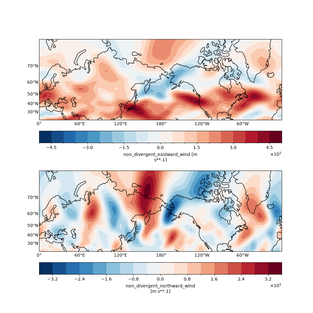
The returned dataset contains upsi and vpsi for the zonal and meridional nondivergent wind components.

uvpsi_fp = ecl.spec.calc_nondivergent_component(
    u_data=uvdata_500_202201["uwnd"],
    v_data=uvdata_500_202201["vwnd"],
)

uvpsi_rs = ecl.spec.calc_nondivergent_component_rs(
    u_data=uvdata_500_202201["uwnd"],
    v_data=uvdata_500_202201["vwnd"],
    transform_backend='latpar',
)

The first figure maps the zonal and meridional nondivergent wind components from the Fortran-backed calculation.

fig, ax = plt.subplots(
    2, 1,
    figsize = (10, 10),
    subplot_kw={"projection": ccrs.Mercator(central_longitude=180)}
)

for axi in ax.flat:
    axi.coastlines()
    axi.gridlines(crs=ccrs.PlateCarree(), draw_labels=["bottom", "left"], alpha = 0)

axi = ax[0]
uvpsi_fp["upsi"].sortby("lat").sel(lat=slice(20, 80)).plot.contourf(
    levels=21,
    ax = axi,
    cbar_kwargs = {'location': 'bottom', 'format': formatter, 'pad': 0.1},
    transform = ccrs.PlateCarree(),
)

axi = ax[1]
uvpsi_fp["vpsi"].sortby("lat").sel(lat=slice(20, 80)).plot.contourf(
    levels=21,
    ax = axi,
    cbar_kwargs = {'location': 'bottom', 'format': formatter, 'pad': 0.1},
    transform = ccrs.PlateCarree(),
)

<cartopy.mpl.contour.GeoContourSet object at 0x7af7a7d02240>

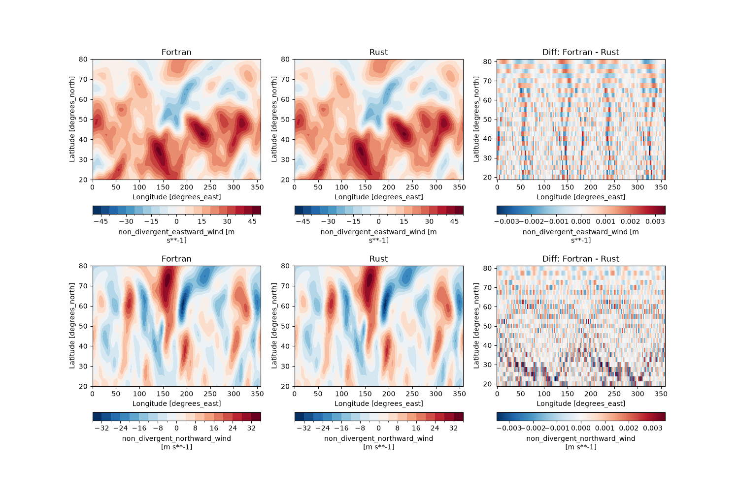
The final figure compares each nondivergent wind component from the two backends and plots the component-wise differences.

fig, ax = plt.subplots(2, 3, figsize = (15, 10))

uvpsi_fp["upsi"].sortby("lat").sel(lat=slice(20, 80)).plot.contourf(
    levels=21,
    ax = ax[0, 0],
    cbar_kwargs = {'location': 'bottom'},
)
ax[0, 0].set_title("Fortran")

uvpsi_rs["upsi"].sortby("lat").sel(lat=slice(20, 80)).plot.contourf(
    levels=21,
    ax = ax[0, 1],
    cbar_kwargs = {'location': 'bottom'},
)
ax[0, 1].set_title("Rust")

(uvpsi_fp["upsi"] - uvpsi_rs["upsi"]).sortby("lat").sel(lat=slice(20, 80)).plot(
    ax = ax[0, 2],
    cbar_kwargs = {'location': 'bottom'},
)
ax[0, 2].set_title("Diff: Fortran - Rust")

uvpsi_fp["vpsi"].sortby("lat").sel(lat=slice(20, 80)).plot.contourf(
    levels=21,
    ax = ax[1, 0],
    cbar_kwargs = {'location': 'bottom'},
)
ax[1, 0].set_title("Fortran")

uvpsi_rs["vpsi"].sortby("lat").sel(lat=slice(20, 80)).plot.contourf(
    levels=21,
    ax = ax[1, 1],
    cbar_kwargs = {'location': 'bottom'},
)
ax[1, 1].set_title("Rust")

(uvpsi_fp["vpsi"] - uvpsi_rs["vpsi"]).sortby("lat").sel(lat=slice(20, 80)).plot(
    ax = ax[1, 2],
    cbar_kwargs = {'location': 'bottom'},
)
ax[1, 2].set_title("Diff: Fortran - Rust")

Text(0.5, 1.0, 'Diff: Fortran - Rust')