easyclimate.physics.moisture
Submodules
Functions
|
Calculate the ambient dew point temperature given the vapor pressure. |
|
Calculate moist adiabatic lapse rate. |
|
Calculate the mixing ratio of a gas. |
|
Calculate the saturation mixing ratio of water vapor. |
|
Calculate the vapor pressure. |
|
Calculate the saturation water vapor (partial) pressure. |
|
Calculate wet-bulb potential temperature using iteration. |
Calculate wet-bulb potential temperature (\(\theta_w\)). |
|
Calculate wet-bulb potential temperature using Robert Davies-Jones (2008) approximation. |
|
|
Calculate wet-bulb temperature using Stull (2011) empirical formula. |
|
Calculate wet-bulb temperature using Sadeghi et. al (2011) empirical formula. |
Package Contents
- easyclimate.physics.moisture.calc_dewpoint(vapor_pressure_data: xarray.DataArray, vapor_pressure_data_units: Literal['hPa', 'Pa', 'mbar']) xarray.DataArray
Calculate the ambient dew point temperature given the vapor pressure.
This function inverts the Bolton (1980) formula for saturation vapor pressure to instead calculate the temperature. This yields the following formula for dewpoint in degrees Celsius, where \(e\) is the ambient vapor pressure in millibars:
\[T = \frac{243.5 \log(e / 6.112)}{17.67 - \log(e / 6.112)}\]Parameters
- vapor_pressure_data:
xarray.DataArray. Water vapor partial pressure.
- vapor_pressure_data_units:
str. The unit corresponding to vapor_pressure_data value. Optional values are hPa, Pa.
Returns
- The dew point ( \(\\mathrm{degC}\) ).
See also
https://unidata.github.io/MetPy/latest/api/generated/metpy.calc.dewpoint.html
Bolton, D. (1980). The Computation of Equivalent Potential Temperature. Monthly Weather Review, 108(7), 1046-1053. https://journals.ametsoc.org/view/journals/mwre/108/7/1520-0493_1980_108_1046_tcoept_2_0_co_2.xml
- vapor_pressure_data:
- easyclimate.physics.moisture.calc_moist_adiabatic_lapse_rate(pressure_data: xarray.DataArray, temperature_data: xarray.DataArray, pressure_data_units: Literal['hPa', 'Pa', 'mbar'], temperature_data_units: Literal['celsius', 'kelvin', 'fahrenheit']) xarray.DataArray
Calculate moist adiabatic lapse rate.
Parameters
- pressure_data:
xarray.DataArray. The pressure data set.
- temperature_data:
xarray.DataArray. Atmospheric temperature.
- pressure_data_units:
str. The unit corresponding to pressure_data value. Optional values are hPa, Pa, mbar.
- temperature_data_units:
str. The unit corresponding to temperature_data value. Optional values are celsius, kelvin, fahrenheit.
Returns:
- dtdp
xarray.DataArray( \(\mathrm{K/hPa}\) ). Moist adiabatic lapse rate.
- pressure_data:
- easyclimate.physics.moisture.calc_mixing_ratio(partial_pressure_data: xarray.DataArray, total_pressure_data: xarray.DataArray, molecular_weight_ratio: float = 0.6219569100577033) xarray.DataArray
Calculate the mixing ratio of a gas.
This calculates mixing ratio given its partial pressure and the total pressure of the air. There are no required units for the input arrays, other than that they have the same units.
Parameters
- partial_pressure_data:
xarray.DataArray. Partial pressure of the constituent gas.
- total_pressure_data:
xarray.DataArray. Total air pressure.
- molecular_weight_ratio
float, optional. The ratio of the molecular weight of the constituent gas to that assumed for air. Defaults to the ratio for water vapor to dry air (\(\epsilon\approx0.622\)).
Note
The units of partial_pressure_data and total_pressure_data should be the same.
Returns
- The mixing ratio ( \(\mathrm{g/g}\) ).
- partial_pressure_data:
- easyclimate.physics.moisture.calc_saturation_mixing_ratio(total_pressure_data: xarray.DataArray, temperature_data: xarray.DataArray, temperature_data_units: Literal['celsius', 'kelvin', 'fahrenheit'], total_pressure_data_units: Literal['hPa', 'Pa', 'mbar']) xarray.DataArray
Calculate the saturation mixing ratio of water vapor.
This calculation is given total atmospheric pressure and air temperature.
Parameters
- total_pressure_data:
xarray.DataArray. Total atmospheric pressure.
- temperature_data:
xarray.DataArray. Atmospheric temperature.
- temperature_data_units:
str. The unit corresponding to temperature_data value. Optional values are celsius, kelvin, fahrenheit.
- total_pressure_data_units:
str. The unit corresponding to total_pressure_data value. Optional values are hPa, Pa.
Returns
- The saturation mixing ratio ( \(\mathrm{g/g}\) ).
- total_pressure_data:
- easyclimate.physics.moisture.calc_vapor_pressure(pressure_data: xarray.DataArray, mixing_ratio_data: xarray.DataArray, pressure_data_units: Literal['hPa', 'Pa', 'mbar'] = None, epsilon: float = 0.6219569100577033) xarray.DataArray
Calculate the vapor pressure.
Parameters
- pressure_data:
xarray.DataArray. The pressure data set.
- mixing_ratio_data:
xarray.DataArray. The mixing ratio of a gas.
- epsilon:
float. The molecular weight ratio, which is molecular weight of the constituent gas to that assumed for air. Defaults to the ratio for water vapor to dry air. (\(\epsilon \approx 0.622\))
- pressure_data_units:
str. The unit corresponding to pressure_data value. Optional values are hPa, Pa.
Returns
- The water vapor (partial) pressure, units according to
pressure_data_units.
- pressure_data:
- easyclimate.physics.moisture.calc_saturation_vapor_pressure(temperature_data: xarray.DataArray, temperature_data_units: Literal['celsius', 'kelvin', 'fahrenheit']) xarray.DataArray
Calculate the saturation water vapor (partial) pressure.
Parameters
- temperature_data:
xarray.DataArray. Atmospheric temperature.
- temperature_data_units:
str. The unit corresponding to temperature_data value. Optional values are celsius, kelvin, fahrenheit.
Returns
- The saturation water vapor (partial) pressure ( \(\mathrm{hPa}\) ).
See also
Bolton, D. (1980). The Computation of Equivalent Potential Temperature. Monthly Weather Review, 108(7), 1046-1053. https://journals.ametsoc.org/view/journals/mwre/108/7/1520-0493_1980_108_1046_tcoept_2_0_co_2.xml
https://unidata.github.io/MetPy/latest/api/generated/metpy.calc.saturation_vapor_pressure.html
- temperature_data:
- easyclimate.physics.moisture.calc_wet_bulb_temperature_iteration(temperature_data: xarray.DataArray, relative_humidity_data: xarray.DataArray, pressure_data: xarray.DataArray, temperature_data_units: Literal['celsius', 'kelvin', 'fahrenheit'], relative_humidity_data_units: Literal['%', 'dimensionless'], pressure_data_units: Literal['hPa', 'Pa', 'mbar'], A: float = 0.662 * 10**-3, tolerance: float = 0.01, max_iter: int = 100, method: Literal['easyclimate-backend', 'easyclimate-rust'] = 'easyclimate-rust') xarray.DataArray
Calculate wet-bulb potential temperature using iteration.
The iterative formula
\[e = e_{tw} - AP(t-t_{w})\]\(e\) is the water vapor pressure
\(e_{tw}\) is the saturation water vapor pressure over a pure flat ice surface at wet-bulb temperature \(t_w\) (when the wet-bulb thermometer is frozen, this becomes the saturation vapor pressure over a pure flat ice surface)
\(A\) is the psychrometer constant
\(P\) is the sea-level pressure
\(t\) is the dry-bulb temperature
\(t_w\) is the wet-bulb temperature
Parameters
- temperature_data:
xarray.DataArray. Atmospheric temperature.
- relative_humidity_data:
xarray.DataArray. The relative humidity.
- pressure_data:
xarray.DataArray. The pressure data set.
- temperature_data_units:
str. The unit corresponding to temperature_data value. Optional values are celsius, kelvin, fahrenheit.
- relative_humidity_data_units:
str. The unit corresponding to vapor_pressure_data value. Optional values are
%,dimensionless.- pressure_data_units:
str. The unit corresponding to pressure_data value. Optional values are hPa, Pa, mbar.
- A:
float. Psychrometer coefficients.
Psychrometer Type and Ventilation Rate
Wet Bulb Unfrozen (10^-3/°C^-1)
Wet Bulb Frozen (10^-3/°C^-1)
Ventilated Psychrometer (2.5 m/s)
0.662
0.584
Spherical Psychrometer (0.4 m/s)
0.857
0.756
Cylindrical Psychrometer (0.4 m/s)
0.815
0.719
Chinese Spherical Psychrometer (0.8 m/s)
0.7949
0.7949
- tolerance:
float. Minimum acceptable deviation of the iterated value from the true value.
- max_iter:
int. Maximum number of iterations.
- method{“easyclimate-backend”,”easyclimate-rust”}
Backend implementation.
Returns
- tw:
xarray.DataArray( \(\mathrm{degC}\) ) Wet-bulb temperature
Examples
>>> import xarray as xr
>>> import numpy as np

# Create sample data
>>> temp = xr.DataArray(np.array([20, 25, 30]), dims=['point'])
>>> rh = xr.DataArray(np.array([50, 60, 70]), dims=['point'])
>>> pressure = xr.DataArray(np.array([1000, 950, 900]), dims=['point'])

# Calculate wet-bulb potential temperature
>>> theta_w = calc_wet_bulb_potential_temperature_iteration(
...     temperature_data=temp,
...     relative_humidity_data=rh,
...     pressure_data=pressure,
...     temperature_data_units="celsius",
...     relative_humidity_data_units="%",
...     pressure_data_units="hPa"
... )

# Example with 2D data
>>> temp_2d = xr.DataArray(np.random.rand(10, 10) * 30, dims=['lat', 'lon'])
>>> rh_2d = xr.DataArray(np.random.rand(10, 10) * 100, dims=['lat', 'lon'])
>>> pres_2d = xr.DataArray(np.random.rand(10, 10) * 200 + 800, dims=['lat', 'lon'])
>>> theta_w_2d = calc_wet_bulb_potential_temperature_iteration(
...     temp_2d, rh_2d, pres_2d, "celsius", "%", "hPa"
... )
See also
Fan, J. (1987). Determination of the Psychrometer Coefficient A of the WMO Reference Psychrometer by Comparison with a Standard Gravimetric Hygrometer. Journal of Atmospheric and Oceanic Technology, 4(1), 239-244. https://journals.ametsoc.org/view/journals/atot/4/1/1520-0426_1987_004_0239_dotpco_2_0_co_2.xml
Wang Haijun. (2011). Two Wet-Bulb Temperature Estimation Methods and Error Analysis. Meteorological Monthly (Chinese), 37(4): 497-502. website: http://qxqk.nmc.cn/html/2011/4/20110415.html
Cheng Zhi, Wu Biwen, Zhu Baolin, et al, (2011). Wet-Bulb Temperature Looping Iterative Scheme and Its Application. Meteorological Monthly (Chinese), 37(1): 112-115. website: http://qxqk.nmc.cn/html/2011/1/20110115.html
Example(s) related to the function
- easyclimate.physics.moisture.calc_wet_bulb_potential_temperature_iteration(temperature_data: xarray.DataArray, relative_humidity_data: xarray.DataArray, pressure_data: xarray.DataArray, temperature_data_units: Literal['celsius', 'kelvin', 'fahrenheit', 'degC', 'degK'], relative_humidity_data_units: Literal['%', 'dimensionless'], pressure_data_units: Literal['hPa', 'Pa', 'mbar'], A: float = 0.000662, tolerance: float = 0.01, max_iter: int = 100, method: Literal['easyclimate-backend', 'easyclimate-rust'] = 'easyclimate-rust') xarray.DataArray
Calculate wet-bulb potential temperature (\(\theta_w\)).
The iterative formula for wet-bulb temperature
\[e = e_{tw} - AP(t-t_{w})\]\(e\) is the water vapor pressure
\(e_{tw}\) is the saturation water vapor pressure over a pure flat ice surface at wet-bulb temperature \(t_w\) (when the wet-bulb thermometer is frozen, this becomes the saturation vapor pressure over a pure flat ice surface)
\(A\) is the psychrometer constant
\(P\) is the sea-level pressure
\(t\) is the dry-bulb temperature
\(t_w\) is the wet-bulb temperature
Wet-bulb potential temperature (\(\theta_w\)) is defined as the temperature that an air parcel would have if it were first brought to saturation at its ambient pressure (i.e., cooled to the wet-bulb temperature, \(T_w\)), and then brought dry-adiabatically to a reference pressure, conventionally (\(p_0 = 1000 \mathrm{hPa}\)).
This quantity is therefore obtained from two steps:
Compute the wet-bulb temperature (\(T_w\)) at the parcel’s pressure (\(p\));
Apply the dry-adiabatic (Poisson) transformation from (\(p\)) to (\(p_0\)).
Under this definition, once (\(T_w\)) is known, (\(\theta_w\)) follows directly as
\[\theta_w = (T_w + 273.15) ( \frac{p_0}{p}) ^{\kappa} - 273.15\]where \(\kappa = \frac{R_d}{c_p} \approx 0.2854\), and \(p_0 = 1000 \mathrm{hPa}\).
This formulation makes clear that the iterative/nonlinear part of the calculation is confined to determining (\(T_w\)); the mapping from (\(T_w\)) to (\(\theta_w\)) is purely algebraic via the dry-adiabatic relation.
Parameters
- temperature_data:
xarray.DataArray. Atmospheric temperature.
- relative_humidity_data:
xarray.DataArray. The relative humidity.
- pressure_data:
xarray.DataArray. The pressure data set.
- temperature_data_units:
str. The unit corresponding to temperature_data value. Optional values are celsius, kelvin, fahrenheit.
- relative_humidity_data_units:
str. The unit corresponding to vapor_pressure_data value. Optional values are
%,dimensionless.- pressure_data_units:
str. The unit corresponding to pressure_data value. Optional values are hPa, Pa, mbar.
- A:
float. Psychrometer coefficients.
Psychrometer Type and Ventilation Rate
Wet Bulb Unfrozen (10^-3/°C^-1)
Wet Bulb Frozen (10^-3/°C^-1)
Ventilated Psychrometer (2.5 m/s)
0.662
0.584
Spherical Psychrometer (0.4 m/s)
0.857
0.756
Cylindrical Psychrometer (0.4 m/s)
0.815
0.719
Chinese Spherical Psychrometer (0.8 m/s)
0.7949
0.7949
- tolerance:
float. Minimum acceptable deviation of the iterated value from the true value.
- max_iter:
int. Maximum number of iterations.
- method{“easyclimate-backend”,”easyclimate-rust”}
Backend implementation.
Notes
\(\theta_w\) is obtained by first computing the wet-bulb temperature (Tw) and then reducing it dry-adiabatically to 1000 hPa.
- easyclimate.physics.moisture.calc_wet_bulb_potential_temperature_davies_jones2008(pressure_data: xarray.DataArray, temperature_data: xarray.DataArray, dewpoint_data: xarray.DataArray, pressure_data_units: Literal['hPa', 'Pa', 'mbar'], temperature_data_units: Literal['celsius', 'kelvin', 'fahrenheit'], dewpoint_data_units: Literal['celsius', 'kelvin', 'fahrenheit']) xarray.DataArray
Calculate wet-bulb potential temperature using Robert Davies-Jones (2008) approximation.
Parameters
- pressure_data:
xarray.DataArray. The pressure data set.
- temperature_data:
xarray.DataArray. Atmospheric temperature.
- dewpoint_data:
xarray.DataArray. The dewpoint temperature.
- pressure_data_units:
str. The unit corresponding to pressure_data value. Optional values are hPa, Pa, mbar.
- temperature_data_units:
str. The unit corresponding to temperature_data value. Optional values are celsius, kelvin, fahrenheit.
- dewpoint_data_units:
str. The unit corresponding to dewpoint_data value. Optional values are celsius, kelvin, fahrenheit.
Returns
- tw:
xarray.DataArray( \(\mathrm{K}\) ) Wet-bulb temperature
See also
Davies-Jones, R. (2008). An Efficient and Accurate Method for Computing the Wet-Bulb Temperature along Pseudoadiabats. Monthly Weather Review, 136(7), 2764-2785. https://doi.org/10.1175/2007MWR2224.1
Knox, J. A., Nevius, D. S., & Knox, P. N. (2017). Two Simple and Accurate Approximations for Wet-Bulb Temperature in Moist Conditions, with Forecasting Applications. Bulletin of the American Meteorological Society, 98(9), 1897-1906. https://doi.org/10.1175/BAMS-D-16-0246.1
Example(s) related to the function
- pressure_data:
- easyclimate.physics.moisture.calc_wet_bulb_temperature_stull2011(temperature_data: xarray.DataArray, relative_humidity_data: xarray.DataArray, temperature_data_units: Literal['celsius', 'kelvin', 'fahrenheit'], relative_humidity_data_units: Literal['%', 'dimensionless']) xarray.DataArray
Calculate wet-bulb temperature using Stull (2011) empirical formula.
\[T_{w} =T\operatorname{atan}[0.151977(\mathrm{RH} \% +8.313659)^{1/2}]+\operatorname{atan}(T+\mathrm{RH}\%)-\operatorname{atan}(\mathrm{RH} \% -1.676331) +0.00391838(\mathrm{RH}\%)^{3/2}\operatorname{atan}(0.023101\mathrm{RH}\%)-4.686035.\]Tip
This methodology was not valid for ambient conditions with low values of \(T_a\) (dry-bulb temperature; i.e., <10°C), and/or with low values of RH (5% < RH < 10%). The Stull methodology was also only valid at sea level.
Parameters
- temperature_data:
xarray.DataArray. Atmospheric temperature.
- relative_humidity_data:
xarray.DataArray. The relative humidity.
- temperature_data_units:
str. The unit corresponding to temperature_data value. Optional values are celsius, kelvin, fahrenheit.
- relative_humidity_data_units:
str. The unit corresponding to vapor_pressure_data value. Optional values are
%,dimensionless.
Returns
- tw:
xarray.DataArray( \(\mathrm{K}\) ) Wet-bulb temperature
See also
Stull, R. (2011). Wet-Bulb Temperature from Relative Humidity and Air Temperature. Journal of Applied Meteorology and Climatology, 50(11), 2267-2269. https://doi.org/10.1175/JAMC-D-11-0143.1
Stull, R. (2011): Meteorology for Scientists and Engineers. 3rd ed. Discount Textbooks, 924 pp. [Available online at https://www.eoas.ubc.ca/books/Practical_Meteorology/, https://www.eoas.ubc.ca/courses/atsc201/MSE3.html]
Knox, J. A., Nevius, D. S., & Knox, P. N. (2017). Two Simple and Accurate Approximations for Wet-Bulb Temperature in Moist Conditions, with Forecasting Applications. Bulletin of the American Meteorological Society, 98(9), 1897-1906. https://doi.org/10.1175/BAMS-D-16-0246.1
Example(s) related to the function
- temperature_data:
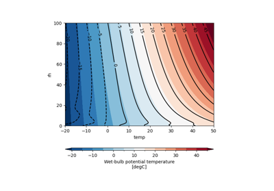
- easyclimate.physics.moisture.calc_wet_bulb_temperature_sadeghi2013(temperature_data: xarray.DataArray, height_data: xarray.DataArray, relative_humidity_data: xarray.DataArray, temperature_data_units: Literal['celsius', 'kelvin', 'fahrenheit'], height_data_units: Literal['m', 'km'], relative_humidity_data_units: Literal['%', 'dimensionless']) xarray.DataArray
Calculate wet-bulb temperature using Sadeghi et. al (2011) empirical formula.
Parameters
- temperature_data:
xarray.DataArray. Atmospheric temperature.
- height_data:
xarray.DataArray. The elevation.
- relative_humidity_data:
xarray.DataArray. The relative humidity.
- temperature_data_units:
str. The unit corresponding to temperature_data value. Optional values are celsius, kelvin, fahrenheit.
- height_data_units:
str. The unit corresponding to height_data value. Optional values are m, km.
- relative_humidity_data_units:
str. The unit corresponding to vapor_pressure_data value. Optional values are
%,dimensionless.
Returns
- tw:
xarray.DataArray( \(\mathrm{degC}\) ) Wet-bulb temperature
See also
Sadeghi, S., Peters, T. R., Cobos, D. R., Loescher, H. W., & Campbell, C. S. (2013). Direct Calculation of Thermodynamic Wet-Bulb Temperature as a Function of Pressure and Elevation. Journal of Atmospheric and Oceanic Technology, 30(8), 1757-1765. https://doi.org/10.1175/JTECH-D-12-00191.1
Example(s) related to the function
- temperature_data: